Chapter 4 Sectoral Structure of Trade
4.1 Package and Data Download
To run the script in this section we again will need the following R packages.
library(tidyverse) # for manipulating data easily
library(readxl) # for reading in data files in a clean format
options(scipen = 100) # turn off scientific notation
For this chapter, we once again will use data from UN Comtrade, but this time we want the data to be disaggregated to the sectoral level (in terms of HS classification, this is the 2-digit HS commodity level).
The sectoral trade flow dataset can be downloaded directly here.
Once the data is downloaded and saved in the appropriate directory, we can clean it. And after that, we can take a look at how the new dataset is structured and what distinct commodity categories are included in the commodity column.
As we look at the structure of the imported dataset in comm object we see that indeed it includes data on per-commodity export and import flows of all economies from and to the World in 2020.
# import the data from the directory containing the downloaded dataset
comm <- read_csv(paste0(data_path, "TradeData_all-world-comm-20.csv"))

# select columns of interest and rename them
comm <- comm %>%
  select(RefYear, ReporterDesc, FlowDesc, PartnerDesc, CmdDesc,
         PrimaryValue, CmdCode)

comm <- comm %>%
  rename(year = RefYear, reporter = ReporterDesc, trade_direction = FlowDesc,
         partner = PartnerDesc,
         commodity = CmdDesc, commodity_code=CmdCode, trade_value_usd = PrimaryValue)

# check the distinct commodity categories
comm %>% distinct(commodity)
## # A tibble: 97 × 1
## commodity
## <chr>
## 1 Animals; live
## 2 Meat and edible meat offal
## 3 Fish and crustaceans, molluscs and other aquatic invertebrates
## 4 Dairy produce; birds' eggs; natural honey; edible products of animal origin,…
## 5 Animal originated products; not elsewhere specified or included
## 6 Trees and other plants, live; bulbs, roots and the like; cut flowers and orn…
## 7 Vegetables and certain roots and tubers; edible
## 8 Fruit and nuts, edible; peel of citrus fruit or melons
## 9 Coffee, tea, mate and spices
## 10 Cereals
## # … with 87 more rows# look at the structure of the dataset
comm## # A tibble: 28,128 × 7
## year reporter trade_direction partner commodity trade_value_…¹ commo…²
## <dbl> <chr> <chr> <chr> <chr> <dbl> <chr>
## 1 2020 Albania Import World Animals; live 26755928. 01
## 2 2020 Albania Export World Animals; live 507085. 01
## 3 2020 Angola Import World Animals; live 9960053. 01
## 4 2020 Angola Export World Animals; live 110490. 01
## 5 2020 Azerbaijan Import World Animals; live 68348203. 01
## 6 2020 Azerbaijan Export World Animals; live 151382. 01
## 7 2020 Argentina Import World Animals; live 23612195. 01
## 8 2020 Argentina Export World Animals; live 15878883. 01
## 9 2020 Australia Import World Animals; live 120534670. 01
## 10 2020 Australia Export World Animals; live 1342439314. 01
## # … with 28,118 more rows, and abbreviated variable names ¹trade_value_usd,
## # ²commodity_codeAt this point we will also load the object where consistent commodity names (at 2-digit level of the HS) are stored to be used in those sections where we will look at index dynamics over a period of time or compare index values across economies.
As was mentioned in the Data access and other considerations section above, while 2-digit commodity codes seem to be consistent throughout the different time periods examined in this Guide, commodity names are not. This is mostly due to the fact that trade flows over different years were reported in different versions of the HS (H0 through to H5), and ideally all commodity codes need to converted to one specific HS version for consistency, which becomes especially relevant if one works with 6-digit level HS codes. However, for the purposes of this section we do not go below 2-digit HS codes. So to make sure that all commodity groups have consistent names throughout we just assigned one commodity name per each 2-digit commodity code disregarding the HS versions reported in the dataset. The dataset with commodity names that we use in this Guide is available here. We only use it in those sections of the Guide where we examine dynamics of a given indicator over several years or compare the indicator values across different economies.
So let’s now clean the dataset to ensure consistency of commodity names in comm object.
# get the csv file with consistent commodity names per each 2-digit commodity code
comm_type <- read_csv(paste0(data_path, "Clean_Commodity_Names.csv") )

# keep commodity and commodity_code columns only
comm_type <- comm_type %>% select(commodity, commodity_code)

# remove commodity column from comm data frame
comm <- comm %>% select(-commodity)

# join the two data frames keeping all the rows of comm data frame
# remove commodity_code column
comm <- left_join(comm, comm_type) %>% select(-commodity_code)

# check new data structure.
# it stayed the same, but commodity names are consistent throughout
comm %>% distinct(commodity)
## # A tibble: 97 × 1
## commodity
## <chr>
## 1 Animals; live
## 2 Meat and edible meat offal
## 3 Fish and crustaceans, molluscs and other aquatic invertebrates
## 4 Dairy produce; birds eggs; natural honey;
## 5 Animal originated products; not elsewhere specified or included
## 6 Trees and other plants, live; bulbs, roots and the like; cut flowers and orn…
## 7 Vegetables and certain roots and tubers; edible
## 8 Fruit and nuts, edible; peel of citrus fruit or melons
## 9 Coffee, tea, mate and spices
## 10 Cereals
## # … with 87 more rowscomm## # A tibble: 28,128 × 6
## year reporter trade_direction partner trade_value_usd commodity
## <dbl> <chr> <chr> <chr> <dbl> <chr>
## 1 2020 Albania Import World 26755928. Animals; live
## 2 2020 Albania Export World 507085. Animals; live
## 3 2020 Angola Import World 9960053. Animals; live
## 4 2020 Angola Export World 110490. Animals; live
## 5 2020 Azerbaijan Import World 68348203. Animals; live
## 6 2020 Azerbaijan Export World 151382. Animals; live
## 7 2020 Argentina Import World 23612195. Animals; live
## 8 2020 Argentina Export World 15878883. Animals; live
## 9 2020 Australia Import World 120534670. Animals; live
## 10 2020 Australia Export World 1342439314. Animals; live
## # … with 28,118 more rows4.2 Competitiveness
What does it tell us? Competitiveness in trade is broadly defined as the capacity of an industry to increase its share in international markets at the expense of its rivals. The competitiveness index is an indirect measure of international market power, evaluated through a country’s share of world markets in selected export categories.
Definition: The index is the share of total exports of a given product from the region under study in total world exports of the same product.
Mathematical definition:
where s is the country of interest, d and w are the set of all countries in the world, i is the sector of interest, and x is the commodity export flow. In words, it is the share of country s’s exports of good i in the total world exports of good i.
Range of values: Takes a value between 0 and 100 per cent, with higher values indicating greater market power of the country in question.
Limitations: The index will vary with the level of data aggregation. Somewhat limited measure of market power, which may depend critically on market structure.
We start our sectoral trade analysis by getting world total export data classified by HS2 commodity code in 2020. In the following chapter we’ll often start from the data frame Xi, eventually filtered by some variables, according to our needs.
After getting our export data it is a good practice to check whether any data points are missing from the dataset. Reshaping data with spread() and gather() functions helps revealing such missing data points. There are different ways to deal with the missing data which we will not discuss here. For the purpose of this Guide, in all such cases below we will assume zero import and export flows for given commodities traded by given economies in a given year. This will not impact our analysis below in any significant manner, as there are very few missing data points for the economies that we will look at as we go through this section.
# keep only export data and three columns of interest
Xi <- comm %>%
  filter(trade_direction == "Export") %>%
  select(reporter, commodity, trade_value_usd)

Xi
## # A tibble: 13,525 × 3
## reporter commodity trade_value_usd
## <chr> <chr> <dbl>
## 1 Albania Animals; live 507085.
## 2 Angola Animals; live 110490.
## 3 Azerbaijan Animals; live 151382.
## 4 Argentina Animals; live 15878883.
## 5 Australia Animals; live 1342439314.
## 6 Austria Animals; live 146762536.
## 7 Bahamas Animals; live 1076
## 8 Bahrain Animals; live 953754.
## 9 Armenia Animals; live 14717057.
## 10 Barbados Animals; live 1551402
## # … with 13,515 more rows# reshape data to reveal if any data on commodity exports is missing
Xi <- Xi %>%
spread(reporter, trade_value_usd) %>%
gather(reporter, trade_value_usd, 2:ncol(.), na.rm = FALSE)
# 1219 out of 14744 data points are revealed to be missing
length(which(is.na(Xi$trade_value_usd)))## [1] 1219# calculate number of missing data points for each economy'
# that have at least one missing data point
check <- Xi %>%
filter(is.na(trade_value_usd)) %>%
group_by(reporter) %>%
summarise(n = n()) %>%
arrange(desc(n))
# look at number of NAs for economies covered in this section
# only Thailand, Philippines and Sri Lanka have few missing data points in 2020
check %>% filter(reporter %in% c("China", "India", "Sri Lanka", "New Zealand",
"Australia", "Thailand", "Viet Nam", "Malaysia", "Indonesia",
"Singapore", "Philippines", "Rep of Korea", "Bangladesh"))## # A tibble: 3 × 2
## reporter n
## <chr> <int>
## 1 Sri Lanka 3
## 2 Philippines 1
## 3 Thailand 1# replace NAs with 0
Xi <- Xi %>%
mutate(trade_value_usd = ifelse(is.na(trade_value_usd), 0, trade_value_usd))
# replacement is successful
anyNA(Xi$trade_value_usd)## [1] FALSESuppose we want to determine the most important economies in world trade in some specific commodities. We can calculate the share of each economy in world trade in those commodities, and rank them. First, let’s make our calculations.
COMP <- Xi

# let's first calculate the share on China's exports of Cotton in total exports of the world
# as we can use that value to later check whether calculations made on a data frame
# containing data on all economies and commodity types are correct

# total world exports of cotton
sum(COMP$trade_value_usd[COMP$commodity=="Cotton"])
## [1] 46569415685# China's exports of cotton
COMP$trade_value_usd[COMP$commodity=="Cotton" & COMP$reporter =="China"] ## [1] 10998836956# China's share in world exports of cotton - 23,62%
COMP$trade_value_usd[COMP$commodity=="Cotton" & COMP$reporter =="China"] / sum(COMP$trade_value_usd[COMP$commodity=="Cotton"]) ## [1] 0.2361816# now let's make calculation for all reporters and all commodities
COMP <- Xi %>%
# group data by commodity
group_by(commodity) %>%
# calculate total world exports of each commodity, ungroup
mutate(total_comm = sum(trade_value_usd, na.rm = T)) %>%
ungroup() %>%
# calculate share of each reporter in world exports of each commodity
# we do not multiply the values by 100 to get percentages,
# as we will need the fractions to calculate positions of sector borders for the pie chart below
mutate(value = trade_value_usd/total_comm) %>%
# select columns of interest
select(reporter, commodity, value)
# let's check the value for China's share in world exports of cotton in this data frame - also 23,62%
COMP$value[COMP$reporter == "China" & COMP$commodity == "Cotton"]## [1] 0.2361816 # round the calculated values
COMP[,"value"] <- round(COMP[,"value"], 4)
# see the resulting dataset structure
COMP %>% filter(reporter == "China") ## # A tibble: 97 × 3
## reporter commodity value
## <chr> <chr> <dbl>
## 1 China Aircraft, spacecraft and parts thereof 0.0112
## 2 China Albuminoids, modified starches, glues, enzymes 0.107
## 3 China Aluminium and articles thereof 0.150
## 4 China Animal or vegetable fats and oils and their cleavage product… 0.0144
## 5 China Animal originated products; not elsewhere specified or inclu… 0.184
## 6 China Animals; live 0.0273
## 7 China Apparel and clothing accessories; knitted or crocheted 0.331
## 8 China Apparel and clothing accessories; not knitted or crocheted 0.335
## 9 China Arms and ammunition, parts and accessories thereof 0.0119
## 10 China Articles of leather; saddlery and harness 0.324
## # … with 87 more rowsNow let’s select one specific commodity - Cotton - and visualize the market shares of the top world exporters in a pie chart.
  # keep the indicator data on Cotton only and arrange data by value from largest to smallest
comp_plot <- COMP %>%
  filter(commodity == "Cotton") %>%
  select(-commodity) %>%
  arrange(desc(value)) %>%
  # keep only the top 5 exporter of cotton in 2020
  slice(1:5)

  # calculate ROW share in exports of cotton
  share_ROW <- 1 - sum(comp_plot$value)

  # add ROW data to comp_plot
  comp_plot <- rbind(comp_plot, c("_ROW", share_ROW))
  comp_plot$value <- as.numeric(comp_plot$value)

comp_plot
## # A tibble: 6 × 2
## reporter value
## <chr> <dbl>
## 1 China 0.236
## 2 USA 0.151
## 3 India 0.125
## 4 Brazil 0.0713
## 5 Viet Nam 0.0581
## 6 _ROW 0.359 # create the plot by
COMP_plot <- comp_plot %>%
# calculating position of each sector boundary on the pie chart
mutate(reporter = factor(reporter, levels = rev(reporter))) %>%
mutate(position = cumsum(lag(value, default = 0)) + value/2) %>%
# creating the pie chart
ggplot(aes(x = "", y = value, fill = reporter)) +
geom_bar(stat = "identity", color = "black") +
coord_polar("y") +
# adding the value labels and title to the chart
geom_text(aes(x = 1.7, y = position, label = paste(value*100, "%"))) +
labs(title = "Top World Exporters of Cotton (2020)", fill = NULL) +
# adjusting the aesthetics of the chart
scale_fill_brewer(palette = "Set1") +
theme_void()
COMP_plot
From the pie chart above we can see that China is the top exporter of cotton in 2020, followed by USA, India, Brazil and Viet Nam.
4.3 Major Export Category
What does it tell us? Major export category is a simple measure of the extent diversification of exports across sectoral categories. If no single category accounts for 50 per cent or more of total exports, the economy is classified as diversified. Identification of dominating products in country’s trade is valuable for both trade policy and adjustment management.
Definition: The index is the value of the largest of sectoral export share in total exports of a given economy.
Mathematical definition:
where s is the country of interest, d is the set of all countries in the world, i is the sector of interest, x is the commodity export flow and X is the total export flow. In words, it is the share of good i in the total exports of country s.
Range of values: Takes a value between 0 and 100 per cent, with higher values indicating greater importance of the product in the export profile of the economy in question.
Limitations: The index will vary with the level of data aggregation. As an indicator of diversification it is limited, one of the others listed below is preferable.
Suppose we want to calculate the share of each commodity in the total exports of China. First, we need to filter all values which have China as reporter in Xi data frame and store results into a new data frame named Xi_CHN. We then make our calculations.
# only keep data on China exports in 2020
Xi_CHN <- Xi[Xi$reporter=="China",]

MEC <- Xi_CHN %>%
  # calculate total export flow of China
  mutate(total = sum(trade_value_usd)) %>%
  # group data by commodity
  group_by(commodity) %>%
  # calculate each commodity shares in total China's exports
  summarize(MEC = trade_value_usd / total ) %>%
  arrange(desc(MEC))

# round the calculated values
MEC$MEC <- round(MEC$MEC,4)

MEC
## # A tibble: 97 × 2
## commodity MEC
## <chr> <dbl>
## 1 Electrical machinery and equipment and parts thereof; sound recorders… 0.274
## 2 Machinery and mechanical appliances; parts thereof 0.17
## 3 Furniture; bedding, mattresses, mattress supports, cushions and simil… 0.0422
## 4 Plastics and articles thereof 0.0372
## 5 Optical, photographic, cinematographic, measuring, checking, medical … 0.031
## 6 Vehicles; other than railway or tramway rolling stock, and parts and … 0.0294
## 7 Textiles, made up articles; sets; worn clothing and worn textile arti… 0.0292
## 8 Toys, games, sports requisites 0.0276
## 9 Iron or steel articles 0.0274
## 10 Apparel and clothing accessories; not knitted or crocheted 0.0241
## # … with 87 more rowsLet’s visualize the values of major commodity exports in a pie chart and express them as a percentages of total China exports.
Nested functions arrange(desc()) help organize MEC values in descending order, and with slice_head(n = 5) we’ll keep only top 5 export categories. We then manually group all other commodities under the label “Other”, calculating their MEC value by doing a subtraction.
Then we add this new observation to mec_plot with rbind(), as we did in the section above.
Finally, we create a pie plot similar to what was done above.
# arrange the data in descending order and
# keep only top 5 largest commodity groups
mec_plot <- MEC %>%
  arrange(desc(MEC)) %>%
  slice_head(n = 5)

# calculate and add data on the share of the remaining commodities in China's exports
mec_plot <- rbind(mec_plot, c("Other", 1 - sum(mec_plot$MEC)))

# using rbind function may turn all data to character strings, so we use as.numeric to turn MEC values into numeric format
mec_plot$MEC <- as.numeric(mec_plot$MEC)
class(mec_plot$MEC)
## [1] "numeric"mec_plot## # A tibble: 6 × 2
## commodity MEC
## <chr> <dbl>
## 1 Electrical machinery and equipment and parts thereof; sound recorders … 0.274
## 2 Machinery and mechanical appliances; parts thereof 0.17
## 3 Furniture; bedding, mattresses, mattress supports, cushions and simila… 0.0422
## 4 Plastics and articles thereof 0.0372
## 5 Optical, photographic, cinematographic, measuring, checking, medical o… 0.031
## 6 Other 0.445# if commodity names are longer than 20 characters, shorten to 20 characters and add ... by
# using str_sub() nested within ifelse()
mec_plot <- mec_plot %>%
mutate(commodity = ifelse(str_length(commodity) > 20,
paste0(str_sub(commodity, 1, 20), "..."),
commodity))
mec_plot## # A tibble: 6 × 2
## commodity MEC
## <chr> <dbl>
## 1 Electrical machinery... 0.274
## 2 Machinery and mechan... 0.17
## 3 Furniture; bedding, ... 0.0422
## 4 Plastics and article... 0.0372
## 5 Optical, photographi... 0.031
## 6 Other 0.445Now let’s create our pie chart.
  # create the plot by
MEC_plot <- mec_plot %>%
  # calculating position of each sector boundary on the pie chart
  mutate(commodity = factor(commodity, levels = rev(commodity))) %>%
  mutate(position = cumsum(lag(MEC, default = 0)) + MEC/2) %>%
  # creating the pie chart
  ggplot(aes(x = "", y = MEC, fill = commodity)) +
  geom_bar(stat = "identity", color = "black") +
  coord_polar("y") +
  # adding the value labels and title to the chart
  geom_text(aes(x = 1.7, y = position, label = paste(MEC*100, "%"))) +
  labs(title = "Top export categories for China (2020)", fill = NULL) +
  # adjusting the aesthetics of the chart
  scale_fill_brewer(palette = "Set1") +
  theme_void()

MEC_plot
From the chart above we see that for China in 2020 the most important export sector included electrical machinery, equipment and appliances, as represented by yellow and orange sectors of the pie chart.
4.4 Sectoral Hirschmann
What does it tell us? The sectoral Hirschmann index is a measure of the sectoral concentration of a region’s exports. It tells us the degree to which a region or country’s exports are dispersed across different economic activities. High concentration levels are sometimes interpreted as an indication of vulnerability to economic changes in a small number of product markets. Over time, decreases in the index may be used to indicate broadening of the export base. An alternative measure is the export diversification index.
Definition: The sectoral Hirschmann index is defined as the square root of the sum of the squared shares of exports of each industry in total exports for the region under study.
Mathematical definition:
where s is the country of interest, d is the set of all countries in the world, i is the sector of interest, x is the commodity export flow and X is the total export flow. Each of the bracketed terms is the share of good i in the exports of country s (see major export category).
Range of values: Takes a value between 0 and 1. Higher values indicate that exports are concentrated in fewer sectors.
Limitations: The Hirschmann index is subject to an aggregation bias.
Let’s go back to Xi object, containing export data for all economies in 2020.
First, we will only keep the export data for the following set of economies: Viet Nam, Thailand, Sri Lanka, Singapore, Philippines, New Zealand, Malaysia, Rep of Korea, Indonesia, India, China, Bangladesh, and Australia. And then we will also calculate and add data on total commodity-wise exports of the rest of the economies (ROW).
SH <- Xi

# create a vector with the names of the countries we're interested in
countries <- c("Viet Nam",
               "Thailand",
               "Sri Lanka",
               "Singapore",
               "Philippines",
               "New Zealand",
               "Malaysia",
               "Rep of Korea.",
               "Indonesia",
               "India" ,
               "China" ,
               "Bangladesh",
               "Australia")

# set aside data on the economies of interest
countries_SH <- SH[SH$reporter %in% countries,]

# keep only the data on the rest of the economies in the dataset
SH <- SH[!(SH$reporter %in% countries),]


SH <- SH %>%
  # group data by commodities
  group_by(commodity) %>%
  # calculate total export values for each commodity, and add _ROW label to this set of values
  summarise(trade_value_usd=sum(trade_value_usd), reporter = '_ROW') %>%
  # arrange columns on the correct order to do rbind later on
  select(reporter, commodity, trade_value_usd)


# bind rest of the world commodity-wise export data to the rest of the dataset
SH <- rbind(countries_SH, SH)

# set aside this cleaned dataset for the use in the following sections
SET_Xi <- SH

SH
## # A tibble: 1,164 × 3
## commodity repor…¹ trade…²
## <chr> <chr> <dbl>
## 1 Aircraft, spacecraft and parts thereof Austra… 1.35e9
## 2 Albuminoids, modified starches, glues, enzymes Austra… 2.60e8
## 3 Aluminium and articles thereof Austra… 2.92e9
## 4 Animal or vegetable fats and oils and their cleavage product… Austra… 4.51e8
## 5 Animal originated products; not elsewhere specified or inclu… Austra… 2.38e8
## 6 Animals; live Austra… 1.34e9
## 7 Apparel and clothing accessories; knitted or crocheted Austra… 9.12e7
## 8 Apparel and clothing accessories; not knitted or crocheted Austra… 1.14e8
## 9 Arms and ammunition, parts and accessories thereof Austra… 1.16e8
## 10 Articles of leather; saddlery and harness Austra… 9.54e7
## # … with 1,154 more rows, and abbreviated variable names ¹reporter,
## # ²trade_value_usdNow let’s calculate the SH index.
Let’s first calculate the SH index for one economy - China. This way we can then check if the calculations performed on the full dataset are correct. Additionally, we will show two options for making such calculation - detailed and consolidated. As was mentioned before, with a step-by-step version of calculation it may be easier to track what is done at each step, which makes it easier to spot errors.
# Option 1: detailed
SH_CHN <- SH %>%
  # keep data on China
  filter(reporter == "China") %>%
        # calculate total export by China
  mutate(totalx = sum(trade_value_usd),
         # calculate share of each commodity in China's total exports
         shx = trade_value_usd/totalx,
         # calculate squared shares of exports of each commodity
         sqr_shx = shx^2,
         # sum the values
         sum_sqr_shx =  sum(sqr_shx),
        # calculate SH for China in 2020
         SH = sqrt(sum_sqr_shx)) %>%
  distinct(reporter, SH)

# SH index is 0.339
SH_CHN$SH
## [1] 0.3389629# Option 2: consolidated
SH_CHN <- SH %>%
# keep data on China
filter(reporter == "China") %>%
# group by reporter
group_by(reporter) %>%
# calculate SH for each reporter
summarize(SH = sqrt(sum((trade_value_usd / sum(trade_value_usd) )^2)))
# SH index is 0.339, same as above
SH_CHN$SH## [1] 0.3389629Now let’s make calculation on a dataset for several reporters.
SH <- SH %>%
  # group by reporter
  group_by(reporter) %>%
  # calculate SH for each reporter
  summarize(SH = sqrt(sum((trade_value_usd / sum(trade_value_usd) )^2)))

# round the values
SH[,2] <- round(SH[,2],2)

SH
## # A tibble: 12 × 2
## reporter SH
## <chr> <dbl>
## 1 _ROW 0.24
## 2 Australia 0.43
## 3 China 0.34
## 4 India 0.21
## 5 Indonesia 0.25
## 6 Malaysia 0.41
## 7 New Zealand 0.33
## 8 Philippines 0.54
## 9 Singapore 0.41
## 10 Sri Lanka 0.34
## 11 Thailand 0.28
## 12 Viet Nam 0.42Let’s create a bar plot to compare the degree of export diversification across a group of examined economies in 2020. For this we again will use ggplot().
Note, that you can adjust the scale values along x-axis with scale_x_continuous() and specify their intervals with breaks =.
# create a bar chart by assigning values to axes, and
# ordering economies by SH values in descending order
SH_plot <- ggplot(SH, aes(x=SH, y=reorder(reporter, SH))) +
  # adding the chart title, removing axis labels
  labs(title = "Sectoral Hirschmann Index for Various Countries (2020)", x = NULL, y = NULL) +
  # adding the bar plot to the chart area, removing legend
  # arranging color code based on values stored in SH from highest to lowest
  geom_bar(aes(fill = desc(SH)), stat='identity', width = 0.5, show.legend = F) +
  # specifying the scale intervals
  scale_x_continuous(breaks = seq(0.0,0.5, by = 0.1)) +
  # applying minimal theme
  theme_minimal()

SH_plot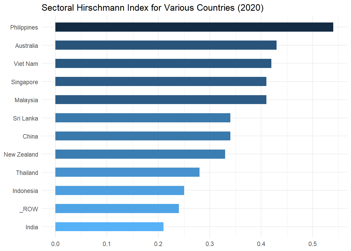
As can be seen from this chart, the most diversified of the examined economies in 2020 were India, Indonesia, and Thailand (and the group of ROW economies), while Philippines was the least diversified economy in the set.
4.5 Export Diversification
What does it tell us? The export diversification index is another measure of the sectoral concentration of a region’s exports. It tells us the degree to which a region or country’s exports are dispersed across different economic activities. Unlike the Hirschmann index, it normalizes the export diversification pattern by comparing it to the world average.
Definition: The sum of the absolute value of the difference between the export category shares of the country under study and the world as a whole, divided by two.
Mathematical definition:
where s is the country of interest, d and w are the set of all countries in the world, i is the sector of interest, x is the commodity export flow and X is the total export flow.
Range of values: Values range from 0 to 1. A value of zero indicates that the export pattern exactly matches the world average. Higher values indicate greater dependence on a small number of products.
Limitations: This measure is subject to an aggregation bias and should be calculated on disaggregated data. An aggregate measure cannot tell us which commodities dominate the export profile, for that we need to go back to the individual shares.
We will now calculate the index for the same group of countries as we did for the Sectoral Hirschmann above. For that we will reuse the SET_Xi object that we created in the previous section.
We will additionally use abs() function to take the absolute value of the difference between per-commodity export shares of each reporter and per-commodity export shares of the world.
# fetch the clean dataset from previous section
ED <- SET_Xi

ED <- ED %>%
  # group data by reporter
  group_by(reporter) %>%
  # calculate export shares of each commodity by distinct reporters,
  # and save values in column ED1
  mutate(ED1 = trade_value_usd / sum(trade_value_usd)) %>%
  # group data by commodity
  group_by(commodity) %>%
  # calculate shares of each commodity in world exports,
  # and save value in column ED2
  mutate(ED2 = sum(trade_value_usd) / sum(SET_Xi$trade_value_usd)) %>%
  # group data by reporter
  group_by(reporter) %>%
  # for each reporter calculate ED index by summing the absolute values of difference
  # between ED1 and ED2 and dividing the result by 2
    summarize(ED = sum(abs(ED1-ED2)) /2)

# round the values
ED[,2] <- round(ED[,2],2)

ED
## # A tibble: 12 × 2
## reporter ED
## <chr> <dbl>
## 1 _ROW 0.08
## 2 Australia 0.64
## 3 China 0.33
## 4 India 0.34
## 5 Indonesia 0.46
## 6 Malaysia 0.37
## 7 New Zealand 0.71
## 8 Philippines 0.46
## 9 Singapore 0.34
## 10 Sri Lanka 0.7
## 11 Thailand 0.28
## 12 Viet Nam 0.48The data is ready to be visualized.
# create a bar chart by assigning values to axes, and
# ordering economies by ED values in descending order
ED_plot <- ggplot(ED, aes(x=ED, y=reorder(reporter, ED))) +
  # adding the chart title
  labs(title = "Export Diversification Index for Various Countries (2020)", x = NULL, y = NULL) +
  # adding the bar plot to the chart area
  # arranging color code based on values stored in ED from highest to lowest
  geom_bar(aes(fill = desc(ED)), stat='identity', width = 0.5, show.legend = F) +
  # applying minimal theme
  theme_minimal()

ED_plot
According to ED index values, in 2020 the least diversified examined economies were New Zealand, Sri Lanka and Australia, and the most diversified economy was Thailand. The results are somewhat different from Sectoral Hirschmann above, as Export Diversification index adjusts for what is “normal” for the world as a whole. Again, as a group, ROW economies have the highest export diversification index.
4.6 Revealed Comparative Advantage
What does it tell us? Comparative advantage underlies economists’ explanations for the observed pattern of inter-industry trade. In theoretical models, comparative advantage is expressed in terms of relative prices evaluated in the absence of trade. Since these are not observed, in practice we measure comparative advantage indirectly. Revealed comparative advantage indices (RCA) use the trade pattern to identify the sectors in which an economy has a comparative advantage, by comparing the country of interests’ trade profile with the world average.
Definition: The RCA index is defined as the ratio of two shares. The numerator is the share of a country’s total exports of the commodity of interest in its total exports. The denominator is share of world exports of the same commodity in total world exports.
Mathematical definition:
where s is the country of interest, d and w are the set of all countries in the world, i is the sector of interest, x is the commodity export flow and X is the total export flow. The numerator is the share of good i in the exports of country s, while the denominator is the share of good i in the exports of the world.
Range of values: Takes a value between 0 and +∞. A country is said to have a revealed comparative advantage if the value exceeds one.
Limitations: The index is affected by anything that distorts the trade pattern, e.g., trade barriers.
Suppose we are interested in the cotton market, and need to determine which economies of interest have a comparative advantage in cotton. For that we will reuse the SET_Xi object that we created in the previous section.
See the notes in the code chunk below for the steps we take to calculate RCA.
# fetch the clean dataset
RCA <- SET_Xi

RCA <- RCA %>%
  # group data by reporter
  group_by(reporter) %>%
  # calculate export shares of each commodity in total exports of each economy, and save values in sh column
  mutate(sh = trade_value_usd / sum(trade_value_usd)) %>%
  # group by commodity
  group_by(commodity) %>%
  # calculate share of each commodity exports in total exports of the world, and save values in wsh column
  mutate(wsh = sum(trade_value_usd) / sum(Xi$trade_value_usd)) %>%
  # only keep data on cotton exports
  filter(commodity=="Cotton") %>%
  # group by reporter
  group_by(reporter) %>%
  # calculate RCA for each reporter by dividing sh by wsh
  summarize(RCA = sh/wsh)

RCA[,2] <- round(RCA[,2],2)
RCA
## # A tibble: 12 × 2
## reporter RCA
## <chr> <dbl>
## 1 _ROW 0.74
## 2 Australia 0.47
## 3 China 1.56
## 4 India 7.75
## 5 Indonesia 1.45
## 6 Malaysia 0.39
## 7 New Zealand 0.03
## 8 Philippines 0.03
## 9 Singapore 0.02
## 10 Sri Lanka 0.51
## 11 Thailand 0.53
## 12 Viet Nam 3.54Now let’s display results in a bar plot. We are looking for values exceeding unity (1).
# create a bar chart by assigning values to axes
RCA_plot <- ggplot(RCA, aes(x=RCA, y=reporter)) +
  # adding the chart title, and removing axis labels
  labs(title = "RCA Index for Cotton (2020)", x = NULL, y = NULL) +
  # adding the bar plot to the chart area, removing legend, and
  # specifying bar color
  geom_bar(fill = "dodgerblue4", stat='identity', width = 0.5, show.legend = F) +
  # specifying the scale intervals
  scale_x_continuous(breaks = seq(0,8, by = 1)) +
  # adding a red vertical line indicating location of 1 on x axis
  geom_vline(xintercept = 1, linetype="dotted",
                color = "red", linewidth=1) +
  # applying minimal theme
  theme_minimal()


RCA_plot
In this case, India, Viet Nam, China, and Indonesia are revealed to have had a comparative advantage in cotton trade in 2020.
4.7 Additive RCA
What does it tell us? The additive RCA (ARCA) index is an alternative to the RCA index. Again, it is used to identify the sectors in which an economy has a comparative advantage, and to track changes over time. Unlike the RCA index, it is symmetric (around zero).
Definition: The ARCA index is defined as the difference of two shares: The share of a country’s total exports of the commodity of interest in its total exports and the share of world exports of the same commodity in total world exports.
Mathematical definition:
where s is the country of interest, d and w are the set of all countries in the world, i is the sector of interest, x is the commodity export flow and X is the total export flow. The first term is the share of good i in the exports of country s, while the second term is the share of good i in the exports of the world.
Range of values: Takes a value between −1 and +1. A country is said to have a revealed comparative advantage if the value exceeds zero.
Limitations: As with RCA, the index is affected by anything that distorts the trade pattern, e.g., trade barriers. It does not identify the source of comparative advantage.
The code is pretty much identical to the previous section. We just make subtraction rather than division.
ARCA <- SET_Xi

ARCA <- ARCA %>%
  # group data by reporter
  group_by(reporter) %>%
  # calculate export shares of each commodity in total exports of each economy, and save values in sh column
  mutate(sh = trade_value_usd / sum(trade_value_usd)) %>%
  # group by commodity
  group_by(commodity) %>%
  # calculate share of each commodity exports in total exports of the world, and save values in wsh column
  mutate(wsh = sum(trade_value_usd) / sum(Xi$trade_value_usd)) %>%
  # only keep data on cotton exports
  filter(commodity=="Cotton") %>%
  # group by reporter
  group_by(reporter) %>%
  # calculate ARCA for each reporter by subtracting wsh from sh and summing the resulting values
  summarize(ARCA = sh-wsh)

ARCA
## # A tibble: 12 × 2
## reporter ARCA
## <chr> <dbl>
## 1 _ROW -0.000701
## 2 Australia -0.00143
## 3 China 0.00153
## 4 India 0.0184
## 5 Indonesia 0.00123
## 6 Malaysia -0.00167
## 7 New Zealand -0.00263
## 8 Philippines -0.00264
## 9 Singapore -0.00267
## 10 Sri Lanka -0.00134
## 11 Thailand -0.00129
## 12 Viet Nam 0.00690Now we are looking for values exceeding zero. We also need to fix x-axis.
# create a bar chart by assigning values to axes
ARCA_plot <- ggplot(ARCA, aes(x=ARCA, y=reporter)) +
  # adding the chart title, and removing axis labels
  labs(title = "Additive RCA Index for Cotton (2020)", x = NULL, y = NULL) +
  # adding the bar plot to the chart area, removing legend and
  # specifying bar color
  geom_bar(fill = 'dodgerblue4', stat='identity', width = 0.5, show.legend = F) +
  # applying minimal theme
  theme_minimal()

ARCA_plot
In this case again, India, Viet Nam, China, and Indonesia are revealed to have had a comparative advantage in cotton trade in 2020.
4.8 Michelaye
What does it tell us? The Michelaye index is a second alternative to the RCA index. Again, it is used to identify the sectors in which an economy has a comparative advantage. Like ARCA, it is symmetric around zero. The difference between Michelaye and ARCA is that the former compares the export pattern of the country under study to the export pattern of the world, while the latter compares the export pattern of the country under study to its own import pattern.
Definition: The Michelaye index is defined as the difference of two shares: The share of a country’s total exports of the commodity of interest in its total exports and the share of the same country’s imports of the same commodity in its total imports.
Mathematical definition:
where s is the country of interest, w is the set of all countries in the world, i is the sector of interest, x is the commodity export flow, X is the total export flow, m the commodity import flow, and M the total import flow. The first term is the share of good i in the exports of country s, while the second term is the share of good i in the imports of country s.
Important Note: The mathematical definition for this index provided in the handbook contains an error. Please refer to the mathematical definition provided in this Guide as the correct one.
Range of values: Takes a value between −1 and +1. A country is said to have a revealed comparative advantage if the value exceeds zero.
Limitations: As with RCA and ARCA, the index is affected by anything that distorts the trade pattern, e.g., trade barriers. It does not identify the source of comparative advantage.
For this indicator we additionally will need data on import flows, that we can extract from comm object that we loaded earlier in this chapter. Similarly to what we did earlier, we will first manipulate the import data to only keep the data for our set of economies of interest, will check and fill any missing data points, and we will also add the calculated data on commodity imports by the rest of the world.
# extract data from predownloaded dataset
Mi <- comm %>%
  filter(trade_direction == "Import") %>%
  select(reporter, commodity, trade_value_usd)

# reshape data to reveal if any data on commodity exports are missing, then replace them with 0
Mi <- Mi %>%
  spread(reporter, trade_value_usd) %>%
  gather(reporter, trade_value_usd, 2:ncol(.), na.rm = FALSE) %>%
  mutate(trade_value_usd = ifelse(is.na(trade_value_usd), 0, trade_value_usd))

# create a vector with the names of the countries we're interested in
countries <- c("Viet Nam",
               "Thailand",
               "Sri Lanka",
               "Singapore",
               "Philippines",
               "New Zealand",
               "Malaysia",
               "Rep of Korea.",
               "Indonesia",
               "India" ,
               "China" ,
               "Bangladesh",
               "Australia")

# set aside data on the economies of interest
countries_Mi <- Mi[Mi$reporter %in% countries,]

# keep only the data on the rest of the economies in the dataset
Mi <- Mi[!(Mi$reporter %in% countries),]

Mi <- Mi %>%
    # group data by commodities
  group_by(commodity) %>%
  # calculate total import values for each commodity,
  # and add _ROW label to this set of values
  summarize(trade_value_usd=sum(trade_value_usd),
         reporter = '_ROW') %>%
  # select only columns of interest and arrange them on the correct order to do rbind later on
  select(reporter, commodity, trade_value_usd)

# bind rest of the world commodity-wise import data to the rest of the dataset
Mi <- rbind(countries_Mi, Mi)

# set aside this cleaned dataset for the use in the following sections
SET_Mi <- Mi

Mi
## # A tibble: 1,164 × 3
## commodity repor…¹ trade…²
## <chr> <chr> <dbl>
## 1 Aircraft, spacecraft and parts thereof Austra… 2.48e9
## 2 Albuminoids, modified starches, glues, enzymes Austra… 3.06e8
## 3 Aluminium and articles thereof Austra… 1.89e9
## 4 Animal or vegetable fats and oils and their cleavage product… Austra… 6.00e8
## 5 Animal originated products; not elsewhere specified or inclu… Austra… 7.77e7
## 6 Animals; live Austra… 1.21e8
## 7 Apparel and clothing accessories; knitted or crocheted Austra… 3.10e9
## 8 Apparel and clothing accessories; not knitted or crocheted Austra… 3.49e9
## 9 Arms and ammunition, parts and accessories thereof Austra… 2.58e8
## 10 Articles of leather; saddlery and harness Austra… 1.22e9
## # … with 1,154 more rows, and abbreviated variable names ¹reporter,
## # ²trade_value_usdWe then calculate both import and export shares of each commodity for each reporter. We use merge to create a new data frame object MIC, which includes both of these values in the same row for each reporter. We filter dataset to only keep data on trade in cotton. And then we calculate Michelaye Index by taking the difference of the two shares. Store results into a new variable MIC with mutate().
# take clean data set on exports
MIC_x <- SET_Xi %>%
  # group by reporters
  group_by(reporter) %>%
  # calculate export shares of each commodity in total exports of each economy
  # and save values in sh_x column
  mutate(sh_x = trade_value_usd / sum(trade_value_usd))

# take clean data set on imports
MIC_m <- SET_Mi %>%
  # group by reporters
  group_by(reporter) %>%
  # calculate import shares of each commodity in total imports of each economy
  # and save values in sh_m column
  mutate(sh_m = trade_value_usd / sum(trade_value_usd))

# merge these two data frames
MIC <- merge(MIC_x[,-3], MIC_m[,-3], by = c("reporter", "commodity"))

as_tibble(MIC)
## # A tibble: 1,164 × 4
## reporter commodity sh_x sh_m
## <chr> <chr> <dbl> <dbl>
## 1 _ROW Aircraft, spacecraft and parts thereof 1.60e-2 9.98e-3
## 2 _ROW Albuminoids, modified starches, glues, enzymes 2.00e-3 1.86e-3
## 3 _ROW Aluminium and articles thereof 9.70e-3 9.88e-3
## 4 _ROW Animal or vegetable fats and oils and their cleavag… 4.75e-3 5.19e-3
## 5 _ROW Animal originated products; not elsewhere specified… 5.73e-4 5.97e-4
## 6 _ROW Animals; live 1.48e-3 1.48e-3
## 7 _ROW Apparel and clothing accessories; knitted or croche… 7.68e-3 1.29e-2
## 8 _ROW Apparel and clothing accessories; not knitted or cr… 7.68e-3 1.29e-2
## 9 _ROW Arms and ammunition, parts and accessories thereof 1.18e-3 8.14e-4
## 10 _ROW Articles of leather; saddlery and harness 3.13e-3 4.21e-3
## # … with 1,154 more rowsMIC <- MIC %>%
# keep only data on cotton trade
filter(commodity=="Cotton") %>%
# calculate MIC for each reporter by subtracting sh_m from sh_x
mutate(MIC = sh_x - sh_m) %>%
# select only columns of interest
select(1,5)
# round the values
MIC[,2]<- round(MIC[,2],4)
MIC ## reporter MIC
## 1 _ROW 0.0007
## 2 Australia 0.0010
## 3 China 0.0002
## 4 India 0.0198
## 5 Indonesia -0.0054
## 6 Malaysia -0.0008
## 7 New Zealand -0.0003
## 8 Philippines -0.0009
## 9 Singapore 0.0000
## 10 Sri Lanka -0.0311
## 11 Thailand -0.0008
## 12 Viet Nam -0.0045Now we can plot the results to compare examined economies.
# create a bar chart by assigning values to axes
MIC_plot <- ggplot(MIC, aes(x=MIC, y=reporter)) +
  # adding the chart title, removing axis labels
  labs(title = "Michelaye Index for Cotton (2020)", x = NULL, y = NULL) +
  # adding the bar plot to the chart area, removing the legend
  # specifying bar color
  geom_bar(fill = "dodgerblue4", stat='identity', width = 0.5, show.legend = F) +
  # applying minimal theme
  theme_minimal()

MIC_plot
According to our calculation of Michelaye index, in 2020 India, Australia, China and Rest of the World revealed a comparative advantage in cotton trade.
4.9 Regional Orientation
What does it tell us? The regional orientation index tells us whether exports of a particular product from the region under study to a given destination are greater than exports of the same product to other destinations. In other words, it measures the importance of intra-regional exports relative to extra-regional exports.
Definition: The index is the ratio of two shares. The numerator is the share of a country’s exports of a given product to the region of interest in total exports to the region. The denominator is the share of a country’s exports of a given product to other countries in total exports to other countries.
Mathematical definition:
where s is the country of interest, d is the set of countries in the regional bloc, w is the set of all countries not in the bloc, i is the sector of interest, x is the commodity export flow, and X is the total export flow. The numerator is the share of good i in the exports of country s to region d, while the denominator is the share of good i in the exports of country s to non-members of region d.
Range of values: Takes a value between 0 and +∞. A value greater than unity implies a regional bias in exports.
Limitations: The index may be affected by many factors, including geographical ones. Because it is based on relative shares, a strong regional orientation may be of little economic significance.
Let’s now calculate sectoral RO indices for the economies that are parties to Australia-New Zealand Closer Economic Relations Trade Agreement (ANZCERTA). We will calculate RO index for 2010 and 2020 to also examine its change over time.
First let’s download the clean dataset from here. As you can see from below, the dataset contains data for all commodities exported by Australia and New Zealand (members of ANZCERTA) to each other and to the WORLD in 2010 and 2020.
# import the dataset
Xi_ANZCERTA <- read_csv(paste0(data_path, "TradeData_AUS-NZL-world-regional-20.csv"))

# select columns of interest
Xi_ANZCERTA <- Xi_ANZCERTA %>%
    select(reporter, partner, year, commodity, trade_value_usd)

# this data set does not have any missing data points,
# so not more cleaning is needed
Xi_ANZCERTA
## # A tibble: 776 × 5
## reporter partner year commodity trade…¹
## <chr> <chr> <dbl> <chr> <dbl>
## 1 Australia World 2020 Animals; live 1.34e 9
## 2 Australia New Zealand 2020 Animals; live 3.44e 7
## 3 Australia World 2020 Meat and edible meat offal 1.01e10
## 4 Australia New Zealand 2020 Meat and edible meat offal 4.54e 7
## 5 Australia World 2020 Fish and crustaceans, molluscs and other… 8.23e 8
## 6 Australia New Zealand 2020 Fish and crustaceans, molluscs and other… 1.11e 7
## 7 Australia World 2020 Dairy produce; birds eggs; natural honey; 1.77e 9
## 8 Australia New Zealand 2020 Dairy produce; birds eggs; natural honey; 4.80e 7
## 9 Australia World 2020 Animal originated products; not elsewher… 2.38e 8
## 10 Australia New Zealand 2020 Animal originated products; not elsewher… 3.62e 6
## # … with 766 more rows, and abbreviated variable name ¹trade_value_usdFirst let’s take a look at a step by step calculation of RO index of Australia’s cotton trade in 2020.
# get regional trade of Australia in cotton in 2020
regtrcott <- Xi_ANZCERTA$trade_value_usd[Xi_ANZCERTA$commodity=="Cotton" &
                                          Xi_ANZCERTA$reporter=="Australia" &
                                          Xi_ANZCERTA$partner=="New Zealand" &
                                          Xi_ANZCERTA$year==2020]
regtrcott
## [1] 2959145# calculate all regional trade of Australia in 2020
regtrall <- sum(Xi_ANZCERTA$trade_value_usd[Xi_ANZCERTA$reporter=="Australia" &
Xi_ANZCERTA$partner=="New Zealand" &
Xi_ANZCERTA$year==2020])
regtrall## [1] 6914472382# calculate trade of Australia in cotton with ROW
rowtrcott <- Xi_ANZCERTA$trade_value_usd[Xi_ANZCERTA$commodity=="Cotton" &
Xi_ANZCERTA$reporter=="Australia" &
Xi_ANZCERTA$partner=="World"&
Xi_ANZCERTA$year==2020] -
Xi_ANZCERTA$trade_value_usd[Xi_ANZCERTA$commodity=="Cotton" &
Xi_ANZCERTA$reporter=="Australia" &
Xi_ANZCERTA$partner=="New Zealand" &
Xi_ANZCERTA$year==2020]
rowtrcott## [1] 312507827# calculate all ROW trade of Australia
rowtrall <- sum(Xi_ANZCERTA$trade_value_usd[Xi_ANZCERTA$reporter=="Australia" &
Xi_ANZCERTA$partner=="World"&
Xi_ANZCERTA$year==2020]) -
sum(Xi_ANZCERTA$trade_value_usd[ Xi_ANZCERTA$reporter=="Australia" &
Xi_ANZCERTA$partner=="New Zealand" &
Xi_ANZCERTA$year==2020])
rowtrall## [1] 238131492405# calculate RO index of Australia's cotton trade in 2020
round((regtrcott/regtrall)/(rowtrcott/rowtrall), 2)## [1] 0.33Now let’s calculate RO index for both Australia’s and New Zealand’s trade in cotton in 2020 and present results in a table for comparison.
RO <- Xi_ANZCERTA %>%
  # keep data for 2020 only
  filter(year==2020) %>%
  # group by reporter
  group_by(reporter) %>%
  # calculate cotton export shares of Australia and New Zealand in trade with each other
  mutate( sh = trade_value_usd[partner!="World" & commodity=="Cotton"] /
            sum(trade_value_usd[partner!="World"]),
  # calculate cotton export shares of Australia and New Zealand in trade with the rest of the world
          wsh = (trade_value_usd[partner=="World" & commodity=="Cotton"] -
                   trade_value_usd[partner!="World" & commodity=="Cotton"]) /
    (sum(trade_value_usd[partner=="World"]) - sum(trade_value_usd[partner!="World"])),
  # calculate RO index for Australia and New Zealand by dividing sh by wsh
         RO_cotton = sh/wsh) %>%
  # only keep data on RO index values for Australia and New Zealand
  distinct(RO_cotton = round(RO_cotton,2))

RO
## # A tibble: 2 × 2
## # Groups: reporter [2]
## reporter RO_cotton
## <chr> <dbl>
## 1 Australia 0.33
## 2 New Zealand 4.66Looking at the values above we can see that New Zealand’s exports of cotton are more regionally biased, as the RO index exceeds value of 1.
We’ll now calculate and visualize RO indices for Australia’s trade in selected commodities in 2010 and 2020 to identify possible regional bias of Australia’s exports to ANZCERTA and to see it’s dynamics over time.
As you go, you can check the accuracy of the step-by-step calculations against the results that we obtained above for Australia’s cotton trade in 2020.
ro_plot <- Xi_ANZCERTA %>%
  # filter data to only contain Australia as reporter
    filter(reporter=="Australia") %>%
  # group by year
  group_by(year) %>%
  # calculate values of Australia's total regional trade and total trade with ROW in 2010 and 2020 and
  # store those in reg_trade_value_usd and row_trade_value_usd columns respectively
  mutate(reg_trade_value_usd=sum(trade_value_usd[partner!="World"]),
         row_trade_value_usd = sum(trade_value_usd[partner=="World"]) -
           reg_trade_value_usd) %>%
  # group by year and commodity
   group_by(year,commodity) %>%
  # calculate shares of distinct Australia's commodities in its total exports to ANZCERTA in 2010 and 2020
   mutate( sh = trade_value_usd[partner!="World"] / reg_trade_value_usd,
  # calculate shares of distinct Australia's commodities in its total exports to partners outside of ANZCERTA (ROW) in 2010 and 2020
           wsh = (trade_value_usd[partner=="World"] - trade_value_usd[partner!="World"]) / row_trade_value_usd ,
  # calculate RO for distinct commodity groups in 2010 and 2020
           RO = sh/wsh) %>%
  # only keep data on RO index values for distinct commodity groups in 2010 and 2020
  select(year, commodity, RO) %>%
  distinct()

# only keep RO data for selected commodity groups
 ro_plot <- ro_plot[ro_plot$commodity %in%
                      c("Cereals","Organic chemicals","Silk","Cotton",
                        "Ceramic products","Glass and glassware",
                        "Pharmaceutical products","Iron and steel",
                        "Aluminium and articles thereof",
                         "Meat and edible meat offal"),]

 # round the values and change data in year column to factors
 ro_plot[,3]<- round(ro_plot[,3],4)
 ro_plot$year <- as.factor(ro_plot$year)

ro_plot  <- ro_plot %>%
  arrange(commodity, year)

ro_plot
## # A tibble: 20 × 3
## # Groups: year, commodity [20]
## year commodity RO
## <fct> <chr> <dbl>
## 1 2010 Aluminium and articles thereof 0.649
## 2 2020 Aluminium and articles thereof 0.546
## 3 2010 Ceramic products 12.7
## 4 2020 Ceramic products 37.8
## 5 2010 Cereals 0.5
## 6 2020 Cereals 0.966
## 7 2010 Cotton 0.0977
## 8 2020 Cotton 0.326
## 9 2010 Glass and glassware 23.9
## 10 2020 Glass and glassware 24.0
## 11 2010 Iron and steel 1.68
## 12 2020 Iron and steel 2.62
## 13 2010 Meat and edible meat offal 0.198
## 14 2020 Meat and edible meat offal 0.156
## 15 2010 Organic chemicals 5.09
## 16 2020 Organic chemicals 1.44
## 17 2010 Pharmaceutical products 3.42
## 18 2020 Pharmaceutical products 3.20
## 19 2010 Silk 3.38
## 20 2020 Silk 25.5Let’s visualize the results with ggplot().
# create a bar chart by assigning values to axes
 RO_plot <- ggplot(ro_plot, aes(fill= year, y= commodity,x= RO)) +
  # adding the chart title, and removing axis labels
   labs(title = "RO Index selected Sectors for Australia/ANZCERTA (2010 vs 2020)", x = NULL, y = NULL) +
  # adding the bar plot to the chart area and keeping legend
   geom_bar(position = "dodge", stat='identity', width = 0.7, show.legend = T ) +
  # adding a black vertical dotted blue line indicating location of 1 on x axis
  geom_vline(xintercept = 1, linetype="dotted",
                color = "black", size=1) +
  # choosing color paletter
  scale_fill_brewer(palette = "Set1" ) +
  # applying minimal theme
  theme_minimal()
## Warning: Using `size` aesthetic for lines was deprecated in ggplot2 3.4.0.
## ℹ Please use `linewidth` instead. RO_plot
According to the chart, regional bias is apparent in 6 out of 10 of the examined commodities. Notably, over the period from 2010 till 2020 regional bias has increased significantly in trade in silk and ceramic products and somewhat in iron and steel. Trade in organic chemicals over the same period became significantly less regionally biased.
4.10 Complementarity
What does it tell us?
The complementarity index is a type of overlap index. It measures the degree to which the export pattern of one country matches the import pattern of another. A high degree of complementarity is assumed to indicate more favorable prospects for a successful trade arrangement. Changes over time may tell us whether the trade profiles are becoming more or less compatible.
Definition: The sum of the absolute value of the difference between the import category shares and the export shares of the countries under study, divided by two. The index is converted to percentage form.
Mathematical definition:
where d is the importing country of interest, s is the exporting country of interest, w is the set of all countries in the world, i is the set of industries, x is the commodity export flow, X is the total export flow, m the commodity import flow, and M the total import flow.
In words, we take the sum of the absolute value of the difference between the sectoral import shares of one country and the sectoral export shares of the other. Dividing by 2 converts this to a number between 0 and 1, with zero indicating all shares matched and 1 indicating none did. Subtracting from one reverses the sign, and multiplying by 100 puts the measure in percentage terms.
Range of values: Takes a value between 0 and 100, with zero indicating no overlap and 100 indicating a perfect match in the import/export pattern.
Limitations: High complementarity indices may be misleading if the countries are geographically distant, or if the size difference in the economies is large (i.e., a match in percentage terms does not imply a match in levels). Aggregation bias.
Let’s return to the objects Mi and Xi containing data on sectoral imports and exports (respectively) of all countries from and to the world in 2020.
We want to find the Complementarity Index between China’s exports and Sri Lanka’s imports, so we consecutively filter export and import datasets by reporter, then extract and merge relevant datasets by commodity types, and then calculate the complementarity index as is shown below.
# get the per-commodity export dataset for 2020
 x <- Xi %>%
  # extract export data for China only
     filter(reporter %in% "China") %>%
    # calculate each commodity's share in total exports of China to the world
   mutate(xsh = trade_value_usd / sum(trade_value_usd))

x
## # A tibble: 97 × 4
## commodity repor…¹ trade…² xsh
## <chr> <chr> <dbl> <dbl>
## 1 Aircraft, spacecraft and parts thereof China 2.46e 9 9.49e-4
## 2 Albuminoids, modified starches, glues, enzymes China 3.41e 9 1.32e-3
## 3 Aluminium and articles thereof China 2.46e10 9.50e-3
## 4 Animal or vegetable fats and oils and their cleavage… China 1.44e 9 5.56e-4
## 5 Animal originated products; not elsewhere specified … China 1.83e 9 7.05e-4
## 6 Animals; live China 6.00e 8 2.32e-4
## 7 Apparel and clothing accessories; knitted or crochet… China 6.22e10 2.40e-2
## 8 Apparel and clothing accessories; not knitted or cro… China 6.23e10 2.41e-2
## 9 Arms and ammunition, parts and accessories thereof China 1.85e 8 7.13e-5
## 10 Articles of leather; saddlery and harness China 2.27e10 8.76e-3
## # … with 87 more rows, and abbreviated variable names ¹reporter,
## # ²trade_value_usd# get the per-commodity import dataset for 2020
m <- Mi %>%
# extract import data for Sri Lanka only
filter(reporter %in% "Sri Lanka") %>%
# calculate each commodity's share in total imports of Sri Lanka from the world
mutate(msh = trade_value_usd / sum(trade_value_usd))
m## # A tibble: 97 × 4
## commodity repor…¹ trade…² msh
## <chr> <chr> <dbl> <dbl>
## 1 Aircraft, spacecraft and parts thereof Sri La… 1.34e7 8.56e-4
## 2 Albuminoids, modified starches, glues, enzymes Sri La… 3.29e7 2.11e-3
## 3 Aluminium and articles thereof Sri La… 1.03e8 6.59e-3
## 4 Animal or vegetable fats and oils and their cleavage… Sri La… 2.09e8 1.34e-2
## 5 Animal originated products; not elsewhere specified … Sri La… 7.32e6 4.69e-4
## 6 Animals; live Sri La… 3.38e6 2.16e-4
## 7 Apparel and clothing accessories; knitted or crochet… Sri La… 5.65e7 3.62e-3
## 8 Apparel and clothing accessories; not knitted or cro… Sri La… 1.02e8 6.53e-3
## 9 Arms and ammunition, parts and accessories thereof Sri La… 4.33e6 2.78e-4
## 10 Articles of leather; saddlery and harness Sri La… 5.27e6 3.38e-4
## # … with 87 more rows, and abbreviated variable names ¹reporter,
## # ²trade_value_usd# merge the two datasets by commodity
COM <- merge(x[,-3],m[,-3], by = "commodity")
head(COM[, -1])## reporter.x xsh reporter.y msh
## 1 China 0.0009491571 Sri Lanka 0.0008560416
## 2 China 0.0013178638 Sri Lanka 0.0021068541
## 3 China 0.0094974561 Sri Lanka 0.0065898763
## 4 China 0.0005558982 Sri Lanka 0.0134148715
## 5 China 0.0007054762 Sri Lanka 0.0004693053
## 6 China 0.0002316116 Sri Lanka 0.0002162809 # calculate trade complementarity index for China exports and Sri Lanka imports
COM <- COM %>%
summarize(COM = (1 -(sum(abs(xsh - msh))/2))*100)
COM <- as.numeric(round(COM,2))
COM## [1] 47.56It would be more informative, however, if we see whether or not the trade of China and Sri Lanka have grown more complementary over time. To do that we can construct the Complementarity Indices over several years and look for changes.
As the first step we need to obtain export and import data for China and Sri Lanka over a period of 10 years. Download this dataset and load it into your session.
#Example 2

# load dataset
Com.CHN_SRI <- read_csv(paste0(data_path, "TradeData_Com.CHN_SRI_11-20.csv") )

# keep the columns of interest
Com.CHN_SRI <- Com.CHN_SRI %>%
  select(reporter, year, trade_value_usd, trade_flow, commodity_code)

# ensure consistent commodity names by using comm_type object created earlier
Com.CHN_SRI <- left_join(Com.CHN_SRI, comm_type) %>%
  select(-commodity_code) %>%
  arrange(commodity, year)

Com.CHN_SRI
## # A tibble: 3,675 × 5
## reporter year trade_value_usd trade_flow commodity
## <chr> <dbl> <dbl> <chr> <chr>
## 1 Sri Lanka 2011 234788196 Import Aircraft, spacecraft and parts th…
## 2 China 2011 13541753022 Import Aircraft, spacecraft and parts th…
## 3 Sri Lanka 2011 9140042 Export Aircraft, spacecraft and parts th…
## 4 China 2011 1630431801 Export Aircraft, spacecraft and parts th…
## 5 Sri Lanka 2012 34112971 Import Aircraft, spacecraft and parts th…
## 6 China 2012 17612975043 Import Aircraft, spacecraft and parts th…
## 7 Sri Lanka 2012 26259949 Export Aircraft, spacecraft and parts th…
## 8 China 2012 1558315928 Export Aircraft, spacecraft and parts th…
## 9 Sri Lanka 2013 46683671 Import Aircraft, spacecraft and parts th…
## 10 China 2013 23181189150 Import Aircraft, spacecraft and parts th…
## # … with 3,665 more rowsFirst, we calculate complementarity indices of China’s exports with Sri Lanka’s imports over this period of time, and then we calculate complementarity indices of Sri Lanka’s exports with China’s imports.
# filter data to only keep export flows from China and import flows to Sri Lanka
# note that we filter out data for 2018, as UN Comtrade does not have 2018 trade data for Sri Lanka
Com.CHN <- Com.CHN_SRI %>%
      filter(reporter %in% "China" & trade_flow == "Export" |
               reporter %in% "Sri Lanka" & trade_flow == "Import" ) %>%
  filter(year != 2018) %>%
  select(-reporter)

# reshape the data frame to have export and import flows in separate columns
Com.CHN <- spread(Com.CHN, trade_flow, trade_value_usd)

# check if reshaping reveals any missing data - no missing data was revealed
anyNA(Com.CHN$Export); anyNA(Com.CHN$Import)
## [1] FALSE## [1] FALSECom.CHN <- Com.CHN %>%
# group data by year
group_by(year) %>%
# calculate shares of each commodity in China's total exports in each year
mutate(sh_x = Export / sum(Export),
# calculate shares of each commodity in Sri Lanka's total imports in each year
sh_m = Import / sum(Import),
# calculate absolute difference between values stored in sh_m and sh_x columns
abs_diff = abs(sh_m - sh_x),
# complete calculation of complementarity indices for China's exports with Sri Lanka's imports in each year
COM = (1-sum(abs_diff)/2)*100) %>%
# only keep values of the calculated indices
distinct(COM)
# label the data
Com.CHN$country <- "China"
Com.CHN## # A tibble: 9 × 3
## # Groups: year [9]
## year COM country
## <dbl> <dbl> <chr>
## 1 2011 41.1 China
## 2 2012 44.8 China
## 3 2013 45.7 China
## 4 2014 42.9 China
## 5 2015 45.4 China
## 6 2016 50.2 China
## 7 2017 47.3 China
## 8 2019 48.0 China
## 9 2020 47.6 China# filter data to only keep export flows from Sri Lanka and import flows to China
# note that we filter out data for 2018, as UN Comtrade does not have 2018 trade data for Sri Lank
Com.SRI <- Com.CHN_SRI %>%
filter(reporter %in% "China" & trade_flow == "Import" | reporter %in% "Sri Lanka" & trade_flow == "Export" ) %>%
filter(year != 2018) %>%
select(-reporter)
# reshape the data frame to have export and import flows in separate columns
Com.SRI <- spread(Com.SRI, trade_flow, trade_value_usd)
# check if reshaping reveals any missing data - some missing data (11 data points) was revealed
# for some commodity exports from Sri Lanka
anyNA(Com.SRI$Export); anyNA(Com.SRI$Import)## [1] TRUE## [1] FALSECom.SRI[which(is.na(Com.SRI$Export)==TRUE),]## # A tibble: 11 × 4
## year commodity Export Import
## <dbl> <chr> <dbl> <dbl>
## 1 2011 Zinc and articles thereof NA 1276502647
## 2 2013 Arms and ammunition, parts and accessories thereof NA 4885501
## 3 2013 Commodities not elsewhere specified NA 104735488097
## 4 2014 Commodities not elsewhere specified NA 82763504585
## 5 2015 Tin; articles thereof NA 325302391
## 6 2016 Commodities not elsewhere specified NA 12910356403
## 7 2017 Commodities not elsewhere specified NA 14685080240
## 8 2017 Tin; articles thereof NA 208780375
## 9 2020 Commodities not elsewhere specified NA 10906754656
## 10 2020 Cork and articles of cork NA 35147681
## 11 2020 Fur skins and artificial fur; manufactures thereof NA 543565651# assume 0 export flows for the missing data
Com.SRI$Export[is.na(Com.SRI$Export)] <- 0
Com.SRI <- Com.SRI %>%
# group data by year
group_by(year) %>%
# calculate shares of each commodity in Sri Lanka's total exports in each year
mutate(sh_x = Export / sum(Export),
# calculate shares of each commodity in China's total imports in each year
sh_m = Import / sum(Import),
# calculate absolute difference between values stored in sh_m and sh_x columns
abs_diff = abs(sh_m - sh_x),
# complete calculation of complementarity indices for Sri Lanka's exports with China's imports in each year
COM = (1-sum(abs_diff)/2)*100) %>%
# only keep values of the calculated indices
distinct(COM)
# label the data
Com.SRI$country <- "Sri Lanka"
Com.SRI## # A tibble: 9 × 3
## # Groups: year [9]
## year COM country
## <dbl> <dbl> <chr>
## 1 2011 14.3 Sri Lanka
## 2 2012 15.7 Sri Lanka
## 3 2013 14.2 Sri Lanka
## 4 2014 19.5 Sri Lanka
## 5 2015 19.4 Sri Lanka
## 6 2016 19.5 Sri Lanka
## 7 2017 21.2 Sri Lanka
## 8 2019 22.3 Sri Lanka
## 9 2020 22.1 Sri LankaAs a last step we bind the two data frames together with rbind() and run ggplot() to display and compare the results.
# combine the two datasets with complementarity indices
com_plot <- rbind(Com.SRI, Com.CHN)

# create a bar chart by assigning values to axes
COM_plot <- ggplot(com_plot, aes(x=year, y=COM, fill=country)) +
  # adding the bar plot to the chart area
  # indicating that values for China and Sri Lanka should be displayed with separate bars
  geom_bar(stat='identity', position='dodge', width = 0.8) +
  # selecting colors to be used for the bars
  scale_fill_manual(values=c('dodgerblue2',  'dodgerblue4')) +
  # adding the chart title, removing axis labels
  labs(title = "Complementarity Indices between China/Sri Lanka (2011-2020)", x = NULL, y = NULL) +
  # rotating year labels to display vertically (at 90 degree angle to the x axis)
  theme(axis.text.x = element_text(angle = 90, hjust = 1)) +
  # adjusting year labels to display them a intervals of one year
  scale_x_continuous(breaks = seq(2011,2020, by = 1)) +
  # applying minimal theme
  theme_minimal()


COM_plot
As can be seen from the chart above, China’s exports are notably more complementary with Sri Lanka’s imports than vice versa. China’s exports have grown somewhat more complementary with Sri Lanka’s imports over the examined period. The similar upward trend is revealed for complementarity of Sri Lanka’s exports with China’s imports.
4.11 Export Similarity
What does it tell us? The export similarity (ES) index is another overlap index. It is designed to measure the degree of similarity between the export profiles of two economies. The more similar the export profiles are, the more likely it is that economies are competitors in global markets. High similarity indices may also indicate limited potential for inter-industry trade with a regional trading arrangement.
Definition: The export similarity index is the sum over export categories of the smaller of the sectoral export shares (as a percentage) of each country under study.
Mathematical definition:
where d and s are the countries of interest, w is the set of all countries in the world, i is the set of industries, x is the commodity export flow, and X is the total export flow. In words, we take the smaller of the sectoral export shares (as a percentage) in each product category, and add them together.
Range of values: Takes a value between 0 and 100 per cent. A value of zero indicates no overlap in the export profiles (the countries are not competitors), a value of 100 indicates perfect overlap.
Limitations: Does not consider the level of exports, only the structure, so may be misleading when the size of the economies considered is very different. Subject to aggregation bias.
Let’s calculate the indicators for China and Sri Lanka again. First, we take Xi object to extract export data for China and Sri Lanka in 2020. And to calculate the ES index we will use min function to keep the lowest values of shares for commodity exports by the examined economies. Then we will sum across all commodities and multiply the resulting value by 100.
ES <- Xi %>%
  # keep export data for China and Sri Lanka in 2020
  filter(reporter %in% c("China", "Sri Lanka"))

ES <- ES %>%
  # group data by reporter
  group_by(reporter) %>%
  # find shares of each commodity in total exports of each economy
  mutate(ES =  trade_value_usd / sum(trade_value_usd)) %>%
  # group by commodity
  group_by(commodity) %>%
  # only keep rows containing the lowest shares in each group
  filter(ES == min(ES))

# sum all resulting values multiply by 100 and round the result
ES <- round(sum(ES$ES)*100,2)

ES
## [1] 27.6Let’s take a look a the dynamics of ES index over 10 year period. To do that we will take the data frame object Com.CHN_SRI that we created in section on complementarity index. It contains data on per-commodity export and import flows by China and Sri Lanka from 2011 through to 2020. So we will need to filter the data to only keep export flows.
es_plot <- Com.CHN_SRI %>%
  # filter to only keep data on export flows
  filter(trade_flow =="Export") %>%
  # filter out data for 2018, since there are no trade data for Sri Lanka available in this year
  filter(year != 2018)

# check for any missing data - revealed missing data for 11 data points for Sri Lanka's exports
check <- es_plot %>%
  spread(reporter, trade_value_usd)
anyNA(check$China); anyNA(check$`Sri Lanka`)
## [1] FALSE## [1] TRUE# assume zero trade flows to fill missing data points
es_plot <- es_plot %>%
spread(reporter, trade_value_usd) %>%
mutate( `Sri Lanka` = ifelse(is.na(`Sri Lanka`), 0, `Sri Lanka`)) %>%
gather(key = "reporter", value = "trade_value_usd", 4:5)
es_plot## # A tibble: 1,746 × 5
## year trade_flow commodity repor…¹ trade…²
## <dbl> <chr> <chr> <chr> <dbl>
## 1 2011 Export Aircraft, spacecraft and parts thereof China 1.63e 9
## 2 2011 Export Albuminoids, modified starches, glues, enzy… China 2.05e 9
## 3 2011 Export Aluminium and articles thereof China 1.86e10
## 4 2011 Export Animal or vegetable fats and oils and their… China 5.44e 8
## 5 2011 Export Animal originated products; not elsewhere s… China 1.84e 9
## 6 2011 Export Animals; live China 5.71e 8
## 7 2011 Export Apparel and clothing accessories; knitted o… China 8.02e10
## 8 2011 Export Apparel and clothing accessories; not knitt… China 6.31e10
## 9 2011 Export Arms and ammunition, parts and accessories … China 1.17e 8
## 10 2011 Export Articles of leather; saddlery and harness China 2.69e10
## # … with 1,736 more rows, and abbreviated variable names ¹reporter,
## # ²trade_value_usdes_plot <- es_plot %>%
# group data by reporter and year
group_by(reporter, year) %>%
# find shares of each commodity in total exports of each economy in each year
mutate(ES = trade_value_usd / sum(trade_value_usd)) %>%
# group data by commodity and year
group_by(commodity, year) %>%
# only keep rows containing the lowest shares of commodity exports in each year
filter(ES == min(ES)) %>%
# group by year
group_by(year) %>%
# for each year finalize calculation of ES index
summarise(ES = sum(ES*100))
es_plot## # A tibble: 9 × 2
## year ES
## <dbl> <dbl>
## 1 2011 26.4
## 2 2012 28.0
## 3 2013 26.6
## 4 2014 30.1
## 5 2015 28.5
## 6 2016 29.3
## 7 2017 28.8
## 8 2019 28.3
## 9 2020 27.6# create a bar chart by assigning values to axes
ES_plot <- ggplot(es_plot, aes(x=year, y=ES)) +
# adding the chart title, removing axis labels
labs(title = "Export Similarity Indices between China/Sri Lanka (2011-2020)", x = NULL, y = NULL) +
# adding the bar plot to the chart area, removing legend,
# specifying bar color
geom_bar(fill="deepskyblue4", stat='identity', width = 0.5, show.legend = F) +
# adjusting year labels to display them at intervals of one year
scale_x_continuous(breaks = seq(2011,2020, by = 1)) +
# applying minimal theme
theme_minimal()
ES_plot
According to the calculation results, China and Sri Lanka do not have particularly similar export profiles, and over the examined time period their export similarity fluctuated slightly.
Additional notes: The index gets biased upward as the commodity data is aggregated. The export similarity index may also be calculated using an alternative formula that is similar to the complementarity index examined above.
4.12 Sectoral IIT
What does it tell us? The sectoral intra-industry trade (IIT) is a measure of the degree to which trade in a particular sector represents intra-industry trade (based on scale economies and/or market structure). By engaging in intra-industry trade, a country can reduce the number of similar goods it produces, and benefit from scale economies. Higher IIT ratios suggest that these sources of gains are being exploited. May also indicate that adjustment costs would be lower with trade expansion.
Definition: One minus the ratio of the absolute value of the difference between exports in a given product category and imports in the same category to the sum of exports and imports in the category.
Mathematical definition:
where s is the country of interest, d is the set of all other countries in the world, i is the sector of interest, x is the commodity export flow, and m the commodity import flow. In the ratio, the numerator is the absolute value of the difference between total exports and total imports in sector i, the denominator is the sum of the total exports and imports in sector i.
Range of values: The index ranges from 0 to 1, with zero indicating pure inter-industry trade, and one indicating pure intra-industry trade.
Limitations: The index is subject to aggregation bias (toward unity), both in terms of sectors and regions. It is not appropriate for measuring changes in intra-industry trade (for that the marginal IIT index examined below should be used).
Let’s calculate sectoral IIT for China for 2020. For that we can extract the required dataset from Com.CHN_SRI object once again.
# extract the required dataset
SIIT <- Com.CHN_SRI %>%
  filter(reporter=="China", year == 2020) %>%
  select(-year) %>%
  # reshape the data to have export and import flows in separate columns
  spread(trade_flow, trade_value_usd)

# check if reshaping of data revealed any missing data points - no missing data revealed
anyNA(SIIT$Import); anyNA(SIIT$Import)
## [1] FALSE## [1] FALSEx## # A tibble: 97 × 4
## commodity repor…¹ trade…² xsh
## <chr> <chr> <dbl> <dbl>
## 1 Aircraft, spacecraft and parts thereof China 2.46e 9 9.49e-4
## 2 Albuminoids, modified starches, glues, enzymes China 3.41e 9 1.32e-3
## 3 Aluminium and articles thereof China 2.46e10 9.50e-3
## 4 Animal or vegetable fats and oils and their cleavage… China 1.44e 9 5.56e-4
## 5 Animal originated products; not elsewhere specified … China 1.83e 9 7.05e-4
## 6 Animals; live China 6.00e 8 2.32e-4
## 7 Apparel and clothing accessories; knitted or crochet… China 6.22e10 2.40e-2
## 8 Apparel and clothing accessories; not knitted or cro… China 6.23e10 2.41e-2
## 9 Arms and ammunition, parts and accessories thereof China 1.85e 8 7.13e-5
## 10 Articles of leather; saddlery and harness China 2.27e10 8.76e-3
## # … with 87 more rows, and abbreviated variable names ¹reporter,
## # ²trade_value_usdSIIT <- SIIT %>%
# group by commodity
group_by(commodity) %>%
# calculate the sectoral IIT index
summarize(SIIT = 1-abs(Export - Import) / (Export + Import))
# shorten commodity names
SIIT <- SIIT %>%
mutate(commodity = ifelse(str_length(commodity) > 20, paste0(str_sub(commodity, 1, 20), "..."), commodity))
SIIT[,2] <- round(SIIT[,2],2)
SIIT## # A tibble: 97 × 2
## commodity SIIT
## <chr> <dbl>
## 1 Aircraft, spacecraft... 0.41
## 2 Albuminoids, modifie... 0.93
## 3 Aluminium and articl... 0.5
## 4 Animal or vegetable ... 0.23
## 5 Animal originated pr... 0.59
## 6 Animals; live 0.97
## 7 Apparel and clothing... 0.11
## 8 Apparel and clothing... 0.14
## 9 Arms and ammunition,... 0.11
## 10 Articles of leather;... 0.35
## # … with 87 more rowsNow we can build a plot which depicts the sectoral intra-industry trade indices for selected commodities in China. Just need to subset specific commodities which you are interested in before running the plot code. In the following example we select a few of them.
# keep index data for selected sectors
 siit_plot <- SIIT[c(1,5,8,11,13,14,21,22,23,28,33,36,37,41,44,76,92, 63,82,83,97),]

# create a bar chart by assigning values to axes and
# ordering the commodities by their SIIT values
 SIIT_plot <- ggplot(siit_plot, aes(x=SIIT, y=reorder(commodity, -SIIT))) +
   # adding the chart title, removing axis labels
   labs(title = "IIT Index for Selected Sectors in China (2020)", x = NULL, y = NULL) +
   # adding the bar plot to the chart are, and
   # specifying bar color based on value of SIIT
   geom_bar(aes(fill = SIIT), stat='identity', width = 0.5, show.legend = F) +
   # applying minimal theme
   theme_minimal()

 SIIT_plot
From the chart above we can see that such commodities as vehicles, cork, and cotton are characterized by the highest IIT indices in 2020 indicating greater role of economies of scale in these sectors.
4.13 Aggregate IIT
What does it tell us? The aggregate intra-industry trade index (AIIT) provides us with an overall measure of the relative importance of intra-industry trade in an economy’s trade profile. As with sectoral IIT, higher ratios suggest that the economies of scale and variety sources of gains are being exploited. Alternatives are the trade overlap index, and the complementarity index (when applied to a single country).
Definition: The trade weighted average of the sectoral IIT indices.
Mathematical definition:
where s is the country of interest, d is the set of all other countries in the world, i is the sector of interest, x is the commodity export flow, m the commodity import flow, X the total export flow, and M the total import flow.
The expression is less complicated than it looks. In words, we take each sectoral IIT index and multiply it by the share of that sector in the total trade of country s. We then sum the weighted IIT indices across all commodities.
Range of values: The index ranges from 0 to 1, with zero indicating pure inter- industry trade, and one indicating pure intra-industry trade.
Limitations: As for sectoral IIT, the index is subject to aggregation bias (toward unity), both in terms of sectors and regions. It is not appropriate for measuring changes in intra-industry trade (the marginal IIT index should be used).
First let’s calculate AIIT for India in 2020. Let’s get a required dataset using comm object to extract 2020 export and import data for India. After that we provide two code scripts for calculating AIIT, the latter showing a step-by-step calculation of all the values that feed into the final AIIT calculation.
# extract the required dataset
AIIT <- comm %>%
  filter(reporter=="India", year == 2020) %>%
  select(-year, -partner) %>%
  # reshape the data to have export and import flows in separate columns
  spread(trade_direction, trade_value_usd)

# check if reshaping data revealed any missing data points -
# no missing data points were revealed
anyNA(AIIT$Import)
## [1] FALSEanyNA(AIIT$Export)## [1] FALSEx## # A tibble: 97 × 4
## commodity repor…¹ trade…² xsh
## <chr> <chr> <dbl> <dbl>
## 1 Aircraft, spacecraft and parts thereof China 2.46e 9 9.49e-4
## 2 Albuminoids, modified starches, glues, enzymes China 3.41e 9 1.32e-3
## 3 Aluminium and articles thereof China 2.46e10 9.50e-3
## 4 Animal or vegetable fats and oils and their cleavage… China 1.44e 9 5.56e-4
## 5 Animal originated products; not elsewhere specified … China 1.83e 9 7.05e-4
## 6 Animals; live China 6.00e 8 2.32e-4
## 7 Apparel and clothing accessories; knitted or crochet… China 6.22e10 2.40e-2
## 8 Apparel and clothing accessories; not knitted or cro… China 6.23e10 2.41e-2
## 9 Arms and ammunition, parts and accessories thereof China 1.85e 8 7.13e-5
## 10 Articles of leather; saddlery and harness China 2.27e10 8.76e-3
## # … with 87 more rows, and abbreviated variable names ¹reporter,
## # ²trade_value_usd# Option 1: consolidated
AIIT_IND1 <- AIIT %>%
# group by reporter
group_by(reporter) %>%
# calculate 2020 AIIT for India
summarise(AIIT = sum( (1- abs(Export - Import) / (Export + Import)) *
( (Export + Import)/( sum(Export) + sum(Import)))))
# Option 2: step by step
AIIT_IND2 <- AIIT %>%
mutate(
# calculate total exports in 2020
sumX = sum(Export),
# calculate total imports in 2020
sumM = sum(Import),
# calculate SIIT indices
SIIT = (1-abs(Export-Import)/(Export + Import)),
# calculate weight to be applied to SIIT indices
weight = ((Export + Import) / (sumX + sumM)),
# apply weights to SIIT indices
w_SIIT = SIIT * weight,
# calculate AIIT for India in 2020
AIIT = sum(w_SIIT)
) %>%
# keep only AIIT index value
group_by(reporter) %>%
distinct(AIIT)
# same AIIT values obtained
AIIT_IND1$AIIT==AIIT_IND2$AIIT## [1] TRUE AIIT <- round(AIIT_IND2$AIIT,2)
AIIT## [1] 0.56Let’s repeat the process to calculate and compare 2020 AIIT indices for a group of selected economies: Viet Nam, Thailand, Sri Lanka, Singapore, Philippines, New Zealand, Malaysia, Rep of Korea., Indonesia, India, China, Bangladesh, Australia and the ROW. And again, as a first step let’s extract our dataset with trade flow values for selected countries and calculate trade flow values for ROW.
# set aside data on the economies of interest
countries_AIIT <- comm %>%
  filter(reporter %in% countries, year == 2020) %>%
  select(-year, -partner)

# keep only the data on the rest of the economies in the dataset
AIIT <- comm %>% filter(!(reporter %in% countries), year == 2020) %>%
  select(-year, -partner)

AIIT <- AIIT %>%
  # group data by commodities
  group_by(commodity, trade_direction) %>%
  # calculate total export values for each commodity, and add _ROW label to this set of values
  mutate(sum=sum(trade_value_usd),
         rep = '_ROW') %>%
  # select only columns of interest and arrange them on the correct order to do rbind later on
  select(rep, commodity, sum) %>%
  # keep only unique rows of data and rename the columns
  unique() %>%
  rename(trade_value_usd = sum, reporter = rep)

# bind rest of the world commodity-wise export data to the rest of the dataset
AIIT <- rbind(countries_AIIT, AIIT)

# reshape the data to have export and import flows in separate columns
AIIT <- spread(AIIT, trade_direction, trade_value_usd)

# check if reshaping data revealed any missing data points
anyNA(AIIT$Import); anyNA(AIIT$Export)
## [1] FALSE## [1] TRUE# fill NAs that appeared in Export column for Sri Lanka (assuming zero trade in this categories)
AIIT$Export[is.na(AIIT$Export)] <- 0
aiit_plot <- AIIT %>%
# group by reporter
group_by(reporter) %>%
# calculate 2020 AIIT for selected economies
summarise(AIIT = sum( (1- abs(Export - Import) / (Export + Import)) *
((Export + Import)/( sum(Export) + sum(Import)))))
aiit_plot## # A tibble: 12 × 2
## reporter AIIT
## <chr> <dbl>
## 1 _ROW 0.925
## 2 Australia 0.311
## 3 China 0.585
## 4 India 0.558
## 5 Indonesia 0.524
## 6 Malaysia 0.777
## 7 New Zealand 0.297
## 8 Philippines 0.631
## 9 Singapore 0.825
## 10 Sri Lanka 0.270
## 11 Thailand 0.665
## 12 Viet Nam 0.664 # create a bar chart by assigning values to axes, and
# reordering reporters by their AIIT values
AIIT_plot <- ggplot(aiit_plot, aes(x=AIIT, y=reorder(reporter, -AIIT))) +
# adding the chart title and removing axis labels
labs(title = "Aggregate IIT Index for Selected Economies (2020)", x = NULL, y = NULL) +
# adding the bar plot to the chart area, removing legend,
# specifying bar color based on value of AIIT
geom_bar(aes(fill = AIIT), stat='identity', width = 0.5, show.legend = F) +
# applying minimal theme
theme_minimal()
# compare the results
AIIT_plot
Highest AIIT indices in 2020 were revealed for Singapore, Malaysia, Thailand, Viet Nam and the Philippines. Sri Lanka, Australia and New Zealand are revealed to have lower AIIT in the examined group. Note the high index for the rest of world category - a product of aggregation bias.
4.14 Marginal IIT
What does it tell us? Evaluating changes in IIT over time needs to be done carefully, because the IIT index can remain constant even as the volume of intra-industry trade expands. The marginal IIT index tells us how much of the change in the volume of trade between two periods is intra-industry trade.
Definition: One minus the ratio of the absolute value of the change in exports in a given product category less the change imports in the same category to the sum of the absolute values of the changes in exports and imports in the category.
Mathematical definition:
where s is the country of interest, w is the set of all countries in the world, i is the sector of interest, x is the commodity export flow, and m the commodity import flow, and ∆ is the change.
In words, the numerator of the ratio is the absolute value of the change in exports in category i less the change in imports in the same category. The denominator is the sum of the absolute values of the changes in export and imports of the same product category. The ratio lies between 0 and 1. Subtracting from one gives us a more natural interpretation, with increasing values indicating more intra-industry trade.
Range of values: The index ranges from 0 to 1, with zero indicating change coming from pure inter-industry trade, and one indicating change coming from pure intra-industry trade.
Limitations: As with the other IIT indices, the index is subject to aggregation bias (toward unity), both in terms of sectors and regions.
In the sectoral IIT index example above we considered how much of China’s trade in various commodities in 2020 can be classified as intra-industry. Now, suppose we want to know how the pattern of intra-industry trade has changed from 2019 to 2020. For that we can calculate the marginal IIT index for the same set of sectors between 2019 and 2020. This will tell us how much of the new trade in that period was intra-industry.
So let’s calculate marginal IIT for China over the period of 2019-2020. For that we can extract the required dataset from Com.CHN_SRI object once again.
We will use spread() function to reshape the data to have export and import flows in two separate columns. And we will use diff() and then abs() functions to calculate the absolute values of change in export and import trade flows for each commodity from 2019 to 2020.
# extract the required dataset
 MIIT <- Com.CHN_SRI %>%
   filter(reporter=="China" & year %in% c(2019,2020)) %>%
  # reshape the data to have export and import flows in separate columns
   spread(trade_flow, trade_value_usd)

MIIT
## # A tibble: 194 × 5
## reporter year commodity Export Import
## <chr> <dbl> <chr> <dbl> <dbl>
## 1 China 2019 Aircraft, spacecraft and parts thereof 3.90e 9 1.93e10
## 2 China 2019 Albuminoids, modified starches, glues, enzymes 3.23e 9 3.68e 9
## 3 China 2019 Aluminium and articles thereof 2.61e10 5.80e 9
## 4 China 2019 Animal or vegetable fats and oils and their c… 1.19e 9 9.93e 9
## 5 China 2019 Animal originated products; not elsewhere spe… 2.39e 9 8.56e 8
## 6 China 2019 Animals; live 5.10e 8 4.98e 8
## 7 China 2019 Apparel and clothing accessories; knitted or … 7.14e10 3.65e 9
## 8 China 2019 Apparel and clothing accessories; not knitted… 6.67e10 4.48e 9
## 9 China 2019 Arms and ammunition, parts and accessories th… 1.42e 8 1.03e 7
## 10 China 2019 Articles of leather; saddlery and harness 2.94e10 3.99e 9
## # … with 184 more rows# first, let's calculate MIIT index for China's trade in live animals
1-(abs(diff(MIIT$Export[MIIT$commodity=="Animals; live"]) -
diff(MIIT$Import[MIIT$commodity=="Animals; live"])) /
(abs(diff(MIIT$Export[MIIT$commodity=="Animals; live"])) +
abs(diff(MIIT$Import[MIIT$commodity=="Animals; live"]))))## [1] 0.7910883# now let's calculate MIIT index for China's trade in all commodities
MIIT <- MIIT %>%
# group by commodity
group_by(commodity) %>%
# calculate the marginal IIT index for each commodity traded by China in 2019-2020
summarize( MIIT = 1-((abs(diff(Export) - diff(Import))) /
(abs(diff(Export)) + abs(diff(Import)))))
# shorten commodity names
MIIT$commodity <- sapply(strsplit(MIIT$commodity, ";"),"[[", 1)
# if commodity names still longer than 20 characters, shorten
MIIT <- MIIT %>%
mutate(commodity = ifelse(str_length(commodity) > 20,
paste0(str_sub(commodity, 1, 20), "..."), commodity))
MIIT[,2] <- round(MIIT[,2],2)
MIIT## # A tibble: 97 × 2
## commodity MIIT
## <chr> <dbl>
## 1 Aircraft, spacecraft... 0.25
## 2 Albuminoids, modifie... 0.87
## 3 Aluminium and articl... 0
## 4 Animal or vegetable ... 0.32
## 5 Animal originated pr... 0.28
## 6 Animals 0.79
## 7 Apparel and clothing... 0.03
## 8 Apparel and clothing... 0
## 9 Arms and ammunition,... 0.01
## 10 Articles of leather 0
## # … with 87 more rowsNow we have our data on MIIT for China in 2019-2020. Let’s visualize it.
# keep index data for selected sectors
 miit <- MIIT[c(1,5,8,11,13,14,21,22,23,28,33,36,37,41,44,76,92, 63,82,83,97),]

# create a bar chart by assigning values to axes and ordering the commodities by their MIIT values
# in ascending order
 MIIT_plot <- ggplot(miit, aes(x= MIIT, y= reorder(commodity, -MIIT))) +
   # adding the chart title, removing axis labels
   labs(title = "Marginal IIT Index for Selected Sectors in India (2019-2020)", x = NULL, y = NULL) +
   # adding the bar plot to the chart area, removing legend, and
   # specifying bar color based on value of MIIT
   geom_bar(aes(fill = MIIT), stat='identity', width = 0.5, show.legend = F) +
    # specifying the scale intervals
   scale_x_continuous(breaks = seq(0,1, by = 0.1)) +
   # applying minimal theme
   theme_minimal()

 MIIT_plot
From the chart above we can see that close to 100% of new trade in zink and related goods between 2019 and 2020 was intra-industry, none of the new trade in vehicles was intra-industry within this same period.
4.15 Aggregate Marginal IIT
What does it tell us?
The aggregate marginal intra-industry trade (AMIIT) index is the marginal equivalent of the aggregate IIT index discussed above. It gives us an overall measure of how much of the overall trade expansion between two periods was intra-industry, and how much was intra-industry.
Definition: The marginal trade share weighted average of the marginal IIT indices for each sector of the economy.
Mathematical definition:
where s is the country of interest, d is the set of all other countries in the world, i is the sector of interest, x is the commodity export flow, m the commodity import flow, & the total export flow, M the total import flow, and ∆ the change operator.
Again, the expression is less complicated than it appears. In words, we take the marginal IIT indices for each sector and multiply them by the shares of the corresponding sectors in the marginal trade of country s (i.e., the total new trade between the periods is considered). We then sum the weighted IIT indices across all commodities.
Range of values: The index ranges from 0 to 1, with zero indicating change coming from pure inter-industry trade, and one indicating change coming from pure intra-industry trade.
Limitations: As with the other IIT indices, the index is subject to aggregation bias (toward unity), both in terms of sectors and regions.
As was done above for AIIT index, first let’s calculate MAIIT for India in 2019-2020. Let’s get a required dataset using comm object to extract 2020 export and import data for India. Additionally, we need to load and extract 2019 export and import data for India as well. The required 2019 dataset is available here.
# extract 2020 trade data for India
AMIIT <- comm %>%
  filter(reporter=="India" & year %in% c(2020))

# load 2019 trade data for India
IND_2019 <- read_csv(paste0(data_path, "TradeData_all-world-comm-19.csv"))

IND_2019 <- IND_2019 %>%
  select("year", "reporter",  "trade_direction",  "partner", "trade_value_usd", "commodity") %>%
  filter(reporter=="India" & year %in% c(2019))

# as you can see the additional 2019 dataset is already organized to have the same structure
names(AMIIT); names(IND_2019)
## [1] "year" "reporter" "trade_direction" "partner"
## [5] "trade_value_usd" "commodity"## [1] "year" "reporter" "trade_direction" "partner"
## [5] "trade_value_usd" "commodity"# combine two datasets together
AMIIT <- rbind(IND_2019, AMIIT)
# reshape data to have two separate columns for import and export flows
AMIIT <- AMIIT %>%
spread(trade_direction, trade_value_usd)Then we make a few interim calculations building up towards calculating sectoral MIIT indices and weights. Then we calculate the MIIT indices and the trade weights for each commodity group with mutate() function. And after that we multiply each marginal IIT index by the appropriate weight to obtain sectoral weighted MIIT indices for India. As the last step we sum all weighted MIIT indices to get a single AMIIT index value for India.
AMIIT <- AMIIT %>%
  #group data by commodity
  group_by(commodity) %>%
  # calculate values for change and absolute change in
  # Exports and Imports of each commodity over 2019-2020
  mutate(
        dX_comm=diff(Export),
        dM_comm=diff(Import),
        dX_comm_abs = abs(diff(Export)),
        dM_comm_abs = abs(diff(Import))) %>%
  # remove redundant columns and keep unique rows only, ungroup data
  select(-year, -Export, -Import, -partner) %>%
  unique() %>%
  ungroup() %>%
  # calculate sums of values stored in columns dX_comm_abs and dM_comm_abs respectively
  mutate(
    dX = sum(dX_comm_abs),
    dM = sum(dM_comm_abs)
  ) %>%
  # group data by commodity
  group_by(commodity) %>%

  mutate(
    # calculate  MIIT indices for each commodity type
    MIIT = (1 - abs(dX_comm - dM_comm)/
              (dX_comm_abs + dM_comm_abs)    ),
    # calculate weights to be applied to each commodity type
    weight = ((dX_comm_abs + dM_comm_abs)/(dX+dM)),
    # calculate weighted MIIT indices for each commodity type
    w_MIIT = MIIT * weight
      )

  # sum weighted MIIT indices to obtain AMIIT index for the examined country
AMIIT_IND <- sum(AMIIT$w_MIIT)

AMIIT_IND
## [1] 0.4858682This value of AMIIT index reveals that close to 50% of India’s new trade in 2020 was generated by intra-industry trade.
Now let’s compare 2019-2020 AMIIT indices for a group of selected economies: Viet Nam, Thailand, Sri Lanka, Singapore, Philippines, New Zealand, Malaysia, Rep of Korea., Indonesia, India, China, Bangladesh, Australia and ROW. And again as a first step let’s extract our datasets for selected economies and generate trade flow values for the rest of the world (ROW) in 2020 and 2019.
# extract 2020 trade data for selected economies
AMIIT_countries <- comm %>%
  filter(reporter %in% countries & year %in% c(2020)) %>%
  spread(reporter, trade_value_usd) %>%
  gather(reporter, trade_value_usd, 5:ncol(.), na.rm = FALSE) %>%
  mutate(trade_value_usd = ifelse(is.na(trade_value_usd), 0, trade_value_usd))

# no NAs revealed
anyNA(AMIIT_countries$trade_value_usd)
## [1] FALSE# extract 2019 trade data for selected economies
AMIIT_countries_2019 <- read_csv(paste0(data_path, "TradeData_all-world-comm-19.csv"))
AMIIT_countries_2019 <- AMIIT_countries_2019 %>%
select("year", "reporter", "trade_direction", "partner", "trade_value_usd", "commodity") %>%
filter(reporter %in% countries & year %in% c(2019)) %>%
spread(reporter, trade_value_usd) %>%
gather(reporter, trade_value_usd, 5:ncol(.), na.rm = FALSE) %>%
mutate(trade_value_usd = ifelse(is.na(trade_value_usd), 0, trade_value_usd))
# no NAs revealed
anyNA(AMIIT_countries_2019$trade_value_usd)## [1] FALSE# as you can see the additional 2019 dataset is already organized
# to have the same structure as 2020 dataset
names(AMIIT_countries)## [1] "year" "trade_direction" "partner" "commodity"
## [5] "reporter" "trade_value_usd"names(AMIIT_countries_2019)## [1] "year" "trade_direction" "partner" "commodity"
## [5] "reporter" "trade_value_usd"# combine two datasets together
AMIIT_countries <- rbind(AMIIT_countries_2019, AMIIT_countries) %>%
select(year, reporter, trade_direction, trade_value_usd, commodity)
# extract 2020 trade data for ROW
AMIIT <- comm %>%
filter(!(reporter %in% countries) & year %in% c(2020)) %>%
spread(reporter, trade_value_usd) %>%
gather(reporter, trade_value_usd, 5:ncol(.), na.rm = FALSE) %>%
mutate(trade_value_usd = ifelse(is.na(trade_value_usd), 0, trade_value_usd))
# extract 2019 trade data for ROW
AMIIT_2019 <- read_csv(paste0(data_path, "TradeData_all-world-comm-19.csv"))
AMIIT_2019 <- AMIIT_2019 %>%
select("year", "reporter", "trade_direction", "partner", "trade_value_usd", "commodity") %>%
filter(!(reporter %in% countries) & year %in% c(2019)) %>%
spread(reporter, trade_value_usd) %>%
gather(reporter, trade_value_usd, 5:ncol(.), na.rm = FALSE) %>%
mutate(trade_value_usd = ifelse(is.na(trade_value_usd), 0, trade_value_usd))
# as you can see the additional 2019 dataset is already organized to have the same structure as 2020 dataset
names(AMIIT)## [1] "year" "trade_direction" "partner" "commodity"
## [5] "reporter" "trade_value_usd"names(AMIIT_2019)## [1] "year" "trade_direction" "partner" "commodity"
## [5] "reporter" "trade_value_usd"# combine two datasets together
AMIIT <- rbind(AMIIT_2019, AMIIT)
# first let's check total ROW exports of live animals in 2020
sum(AMIIT$trade_value_usd[AMIIT$year==2020 & AMIIT$trade_direction=="Export" & AMIIT$commodity=="Animals; live"])## [1] 18670450395# let's check total ROW imports of live animals in 2019
sum(AMIIT$trade_value_usd[AMIIT$year==2019 & AMIIT$trade_direction=="Import" & AMIIT$commodity=="Animals; live"])## [1] 20388610922# let's calculate total ROW exports and imports of each commodity in 2019 and 2020
AMIIT <- AMIIT %>%
# group data by year, commodity, trade_direction
group_by(year, commodity, trade_direction) %>%
# calculate total export and import values for each commodity in each year, and add _ROW label to this set of values
mutate(sum=sum(trade_value_usd),
rep = '_ROW') %>%
# select only columns of interest and arrange them on the correct order to do rbind later on
select(rep, commodity, sum) %>%
# keep only unique rows of data and rename and arrange the columns
unique() %>%
rename(trade_value_usd = sum, reporter = rep) %>%
select("year", "reporter", "trade_direction", "trade_value_usd", "commodity")
# check that the values match our earlier calculations
AMIIT$trade_value_usd[AMIIT$year==2020 & AMIIT$trade_direction=="Export" & AMIIT$commodity=="Animals; live"]## [1] 18670450395AMIIT$trade_value_usd[AMIIT$year==2019 & AMIIT$trade_direction=="Import" & AMIIT$commodity=="Animals; live"]## [1] 20388610922# check two dataset structures
names(AMIIT)## [1] "year" "reporter" "trade_direction" "trade_value_usd"
## [5] "commodity"names(AMIIT_countries)## [1] "year" "reporter" "trade_direction" "trade_value_usd"
## [5] "commodity"# bind rest of the world commodity-wise export data to the rest of the dataset
AMIIT <- rbind(AMIIT_countries, AMIIT)
# reshape data to have two separate columns for import and export flows
AMIIT <- AMIIT %>%
spread(trade_direction, trade_value_usd)Now we are ready to calculate and compare AMIIT indices for the selected economies and ROW. We follow the same steps as above while making sure that grouping of values is done to reflect the additional set of countries added to the dataset.
Once calculations are over, check to see that AMIIT index calculated for India in this section is the same as the one we obtained in the section above where we calculated AMIIT index for one country only.
AMIIT <- AMIIT %>%
  #group data by commodity
  group_by(reporter, commodity) %>%
  # calculate values for change and absolute change in Exports and Imports of each commodity over 2019-2020
  mutate(
        dX_comm=diff(Export),
        dM_comm=diff(Import),
        dX_comm_abs = abs(diff(Export)),
        dM_comm_abs = abs(diff(Import))) %>%
  # remove rows where  dX_comm and dM_comm for a given reporter-commodity pair
  # are equal to 0. if you look at the data, you will see that these rows correspond with the
  # missing data points which we filled with zeros, and which thus far ended up having zeros
  # in both import and export flows in both 2019 and 2020
  # if you look at the formula, you will see that these data points will cause issues with
  # the calculation results for Thailand and Philippines
  # (remove this step and see what happens)
  filter(dX_comm != 0 & dM_comm != 0) %>%
  # remove redundant columns and keep unique rows only, ungroup data
  select(-year, -Export, -Import) %>%
  unique() %>%
  group_by(reporter) %>%
  # calculate sums of values stored on columns dX_comm_abs and dM_comm_abs respectively
  mutate(
    dX = sum(dX_comm_abs),
    dM = sum(dM_comm_abs)
  ) %>%
  # group data by commodity
  group_by(reporter, commodity) %>%

  mutate(
    # calculate  MIIT indices for each commodity type
    MIIT = (1 - abs(dX_comm - dM_comm)/
              (dX_comm_abs + dM_comm_abs)    ),
    # calculate weights to be applied to each commodity type
    weight = ((dX_comm_abs + dM_comm_abs)/(dX+dM)),
    # calculate weighted MIIT indices for each commodity type
    w_MIIT = MIIT * weight
      ) %>%
  group_by(reporter) %>%
  mutate(AMIIT = sum(w_MIIT)) %>%
  distinct(AMIIT)

   AMIIT
## # A tibble: 12 × 2
## # Groups: reporter [12]
## reporter AMIIT
## <chr> <dbl>
## 1 _ROW 0.847
## 2 Australia 0.385
## 3 China 0.270
## 4 India 0.486
## 5 Indonesia 0.434
## 6 Malaysia 0.555
## 7 New Zealand 0.196
## 8 Philippines 0.373
## 9 Singapore 0.737
## 10 Sri Lanka 0.169
## 11 Thailand 0.394
## 12 Viet Nam 0.511If you compare the calculated AMIIT value for India with the value obtained in the example above, you will see that they are the same.
Let’s now plot the calculated AMIIT indices for all of the examined economies and the ROW.
AMIIT_plot <- AMIIT
 # create a bar chart by assigning values to axes, and
 # reordering reporters by their AMIIT values
 AMIIT_plot <- ggplot(AMIIT_plot, aes(x=AMIIT, y=reorder(reporter, -AMIIT))) +
 # adding the chart title, and removing axis labels
   labs(title = "Aggregate marginal IIT Index for Selected Economies (2019-2020)", x = NULL, y = NULL) +
 # adding the bar plot to the chart area, removing legend
  # specifying bar color based on value of AMIIT
   geom_bar(aes(fill = AMIIT), stat='identity', width = 0.5, show.legend = F) +
# applying minimal theme
   theme_minimal()

 AMIIT_plot
The graph above reveals that in 2020 intra-industry trade contributed most significantly to new trade of Singapore, Malaysia and Viet Nam (over 50%). Note again the high index for the ROW category - a product of aggregation bias.
4.16 Trade Overlap
What does it tell us?
The trade overlap index is an alternative to the aggregate IIT index. Again, it can tell us about the overall significance of intra-industry trade relative to inter-industry trade in the trade profile of an economy at a point in time. It is marginally easier to calculate than the aggregate IIT index.
Definition: For a given country, the sum over all sectors of the smaller of exports and imports in that sector (the overlap) multiplied by two, as a fraction of the total trade of that country.
Mathematical definition:
where s is the country of interest, w is the set of all countries in the world, i is the sector of interest, x is the commodity export flow, X is the total export flow, m the commodity import flow, and M the total import flow.
The first term is the share of good i in the exports of country s, while the second term is the share of good i in the imports of the world. In words, the numerator measures the overlap of imports and exports, the denominator expresses the overlap as a fraction of total trade.
Range of values: The index ranges from 0 to 1, with zero indicating pure inter-industry trade, and one indicating pure intra-industry trade.
Limitations: Same as for aggregate IIT, the index is subject to aggregation bias (toward unity), both in terms of sectors and regions. It is not appropriate for measuring changes in intra-industry trade (where the marginal IIT index should be used).
Let’s now calculate Trade Overlap index for China in 2020. We get data China’s export and import flows in 2020 from Com.CHN_SRI object.
 TO <- Com.CHN_SRI %>%
  # extract the required dataset
   filter(year == 2020 & reporter == "China" )  %>%
  # reshape the data to have export and import flows in separate columns
   spread(trade_flow, trade_value_usd)

 TO
## # A tibble: 97 × 5
## reporter year commodity Export Import
## <chr> <dbl> <chr> <dbl> <dbl>
## 1 China 2020 Aircraft, spacecraft and parts thereof 2.46e 9 9.40e 9
## 2 China 2020 Albuminoids, modified starches, glues, enzymes 3.41e 9 3.92e 9
## 3 China 2020 Aluminium and articles thereof 2.46e10 8.15e 9
## 4 China 2020 Animal or vegetable fats and oils and their c… 1.44e 9 1.13e10
## 5 China 2020 Animal originated products; not elsewhere spe… 1.83e 9 7.62e 8
## 6 China 2020 Animals; live 6.00e 8 6.35e 8
## 7 China 2020 Apparel and clothing accessories; knitted or … 6.22e10 3.51e 9
## 8 China 2020 Apparel and clothing accessories; not knitted… 6.23e10 4.74e 9
## 9 China 2020 Arms and ammunition, parts and accessories th… 1.85e 8 1.06e 7
## 10 China 2020 Articles of leather; saddlery and harness 2.27e10 4.82e 9
## # … with 87 more rowsFirst we will take the smaller value between exports and imports for each category using min() function. We will then sum the values and multiply those by 2 to get the numerator. The denominator is total trade, Export plus Import. The ratio of these two values gives us the Trade Overlap index.
TO <- TO %>%
  # group by commodity
   group_by(commodity) %>%
  # for each commodity select export or import flow, whichever is smaller
   mutate(TO = (min(Export, Import)))

# calculate the TO index value, and round it
 TO <- 2*sum(TO$TO) / (sum(TO$Export) + sum(TO$Import))
 TO <- round(TO,2)

 TO
## [1] 0.59As is suggested in the handbook, to see how the various available measures of aggregate intra-industry trade compare, we now will take a look at the trade overlap index, the aggregate intra-industry trade index, and the complementarity index values for China.
He have just calculated TO for China in 2020. In section of Aggregate IIT we have already calculated AIIT index for China in 2020 which is now stored in aiit_plot object.
At this point we need to calculate the complementarity index, as a fraction rather than a percentage, with China as both the exporting and importing country. Let’s get the same set of data on China.
 II_COMP <- Com.CHN_SRI %>%
  # extract the required dataset
   filter(year == 2020 & reporter == "China" )  %>%
  # reshape the data to have export and import flows in separate columns
   spread(trade_flow, trade_value_usd)

II_COMP
## # A tibble: 97 × 5
## reporter year commodity Export Import
## <chr> <dbl> <chr> <dbl> <dbl>
## 1 China 2020 Aircraft, spacecraft and parts thereof 2.46e 9 9.40e 9
## 2 China 2020 Albuminoids, modified starches, glues, enzymes 3.41e 9 3.92e 9
## 3 China 2020 Aluminium and articles thereof 2.46e10 8.15e 9
## 4 China 2020 Animal or vegetable fats and oils and their c… 1.44e 9 1.13e10
## 5 China 2020 Animal originated products; not elsewhere spe… 1.83e 9 7.62e 8
## 6 China 2020 Animals; live 6.00e 8 6.35e 8
## 7 China 2020 Apparel and clothing accessories; knitted or … 6.22e10 3.51e 9
## 8 China 2020 Apparel and clothing accessories; not knitted… 6.23e10 4.74e 9
## 9 China 2020 Arms and ammunition, parts and accessories th… 1.85e 8 1.06e 7
## 10 China 2020 Articles of leather; saddlery and harness 2.27e10 4.82e 9
## # … with 87 more rowsNow let’s take a look at the revised formula that is suitable for our task and make the calculations accordingly:
Below we provide two script options: consolidated and step-by-step.
# Option 1: consolidated

 II_COMP1 <- II_COMP  %>%
  # group by reporter
   group_by(reporter) %>%
  # summarize by calculating intra-industry complementarity index
   summarise(
     II_COMP = (1-sum(abs( (Import/sum(Import)) - (Export/sum(Export))  ) ) / 2)

   )

II_COMP2 <- II_COMP %>%
          # calculate sum of all exports
  mutate(sumX = sum(Export),
          # calculate sum of all imports
         sumM = sum(Import),
         # calculate share of each commodity in total exports
         shX = Export/sumX,
         # calculate share of each commodity in total imports
         shM = Import/sumM,
         # find absolute values of difference between import and export shares for each commodity
         diffMX = abs(shM - shX),
         # sum all values in column  diffMX
         sumdiffMX = sum(diffMX),
         # divide value in column sumdiffMX by 2 and subtract it from 1
         II_COMP = 1 - sumdiffMX / 2) %>%
  # group by reporter
  group_by(reporter) %>%
  # only keep intra-industry complementarity index value for China in 2020
  distinct(II_COMP)

# check if the results of the two calculations are the same
II_COMP1$II_COMP==II_COMP2$II_COMP
## [1] TRUE# round the value
II_COMP <- round(II_COMP1$II_COMP,2)
II_COMP ## [1] 0.63Now that we have values of the three indicators available, let’s compare them on a chart.
# compile index values in one data frame
comparison_plot <- data.frame( "Indicator" = c("Trade Overlap","Aggregate IIT",  "Complementarity"),
                               "Value" = c(TO, aiit_plot$AIIT[aiit_plot$reporter=="China"], II_COMP ))


 # create a bar chart by assigning values to axes and ordering the indicators by their value
COMPARISON_plot <- ggplot(comparison_plot, aes(x= Value, y= reorder(Indicator, - Value))) +
  # adding the chart title, removing axis labels
  labs(title = "Comparison of Aggregate Measures of IIT for China (2020)", x = NULL, y = NULL) +
  # adding the bar plot to the chart area, removing legend
  geom_bar(fill = "dodgerblue4", stat='identity', width = 0.5, show.legend = F) +
  # applying minimal theme
  theme_minimal()


COMPARISON_plot
There is slight variation between these three aggregate measures of intra-industry trade calculated to capture the importance of intra-industry trade for China in 2020.