Chapter 3 Direction of Trade

3.1 Data Download

Before we start, let’s load the necessary R packages and turn off scientific notation.

library(tidyverse) # for manipulating data easily
library(readxl) # for reading in data files in a clean format
options(scipen = 100) # turn off scientific notation

For this chapter, we’re going to use the dataset downloaded from UN Comtrade, which covers all export and import flows between all reporters and partners over the period of 2014-2020. The dataset can be downloaded here.

Set the correct path to your directory and save the downloaded dataset there.

data_path <- "your/path/to/data/"

After that, read the dataset into your R session and then take a look at it before you go on to calculating the trade indices described in this section.

# read the dataset into your R session
data <- read_csv(paste0(data_path, "Section3_dataset.csv"))

data

## # A tibble: 394,652 × 6
##     ...1 reporter partner             trade_value_usd  year trade_flow
##    <dbl> <chr>    <chr>                         <dbl> <dbl> <chr>     
##  1     1 Albania  Algeria                          63  2020 Export    
##  2     2 Albania  Algeria                    21704831  2020 Import    
##  3     3 Albania  American Samoa                  515  2020 Import    
##  4     4 Albania  Angola                        52577  2020 Export    
##  5     5 Albania  Anguilla                        206  2020 Export    
##  6     6 Albania  Anguilla                      32206  2020 Import    
##  7     7 Albania  Antarctica                     2293  2020 Import    
##  8     8 Albania  Antigua and Barbuda          476916  2020 Import    
##  9     9 Albania  Areas, nes                  1259118  2020 Export    
## 10    10 Albania  Areas, nes                  2994230  2020 Import    
## # … with 394,642 more rows

3.2 Export Share

What does it tell us? The export share tells us how important a particular export partner is in terms of the overall export profile of an economy. Changes in the export share over time may indicate that the economies in question are becoming more integrated. In the case of intra-regional export shares, increases in the value over time are sometimes interpreted as an indicator of the significance of a regional trading bloc if one exists, or as a measure of potential if one is proposed. The latter assumes that groups with high shares are in some sense ‘natural’ trading partners.

Definition: The export share is the percentage of exports from the region under study (the source) to the region of interest (the destination) in the total exports of the source region.

Mathematical definition

\(XS = \frac{\sum_{sd} X_{sd}}{\sum_{sw} X_{sw}}\times100\)

where s is the set of countries in the source, d is the set of countries in the destination, w is the set of countries in the world, and X is the bilateral total export flow. The numerator is thus exports from the source to the destination, the denominator is total exports from the source.

Range of values: Takes a value between 0 and 100 per cent, with higher values indicating greater importance of selected trading partner.

Limitations: The intra-regional export share is increasing in the size of the bloc considered by definition, so comparing the shares across different blocs may be misleading. High or low export shares and changes over time may reflect factors other than trade policy.

First of all let’s get our trade data for the selected ASEAN-6 economies: Indonesia, Malaysia, Philippines, Thailand, Singapore, and Viet Nam, and then keep only data on export flows in 2020. As we are trying to find total intra-regional trade, we’ll keep 6 selected ASEAN economies as partners plus “World”.

# create a vector with names of ASEAN-6 economies
ASEAN.6 <-  c("Indonesia", "Malaysia", "Philippines", 
              "Singapore", "Thailand", "Viet Nam")

# filter dataset to keep only export flows from ASEAN-6 reporters to ASEAN-6 partners and their total exports to World in 2020
X_ASEAN <- data %>% filter(reporter %in% ASEAN.6 &  
                             year %in% 2020 & 
                             trade_flow == "Export" &
                             partner %in% c(ASEAN.6, "World") & 
                           year == "2020") 

# select variables of interest
XS <- X_ASEAN %>% select(reporter, partner, trade_value_usd, year)

XS

## # A tibble: 36 × 4
##    reporter  partner     trade_value_usd  year
##    <chr>     <chr>                 <dbl> <dbl>
##  1 Indonesia Malaysia         8098764319  2020
##  2 Indonesia Philippines      5900740847  2020
##  3 Indonesia Singapore       10661853725  2020
##  4 Indonesia Thailand         5110298724  2020
##  5 Indonesia Viet Nam         4941357726  2020
##  6 Indonesia World          163191837261  2020
##  7 Malaysia  Indonesia        7039109596  2020
##  8 Malaysia  Philippines      4188601349  2020
##  9 Malaysia  Singapore       33816086225  2020
## 10 Malaysia  Thailand        10786175493  2020
## # … with 26 more rows

Let’s calculate the percentage of ASEAN-6 exports to ASEAN-6 region in total ASEAN-6 exports to the World.

# calculate the indicator, and round the value
XS <- XS %>% 
  summarize(XS = sum(trade_value_usd[partner!="World"]) / 
              sum(trade_value_usd[partner=="World"])*100)
XS <- round(XS, 2)

XS

## # A tibble: 1 × 1
##      XS
##   <dbl>
## 1  19.0

Now let’s calculate the same indicator for the same regional bloc but for a series of 5 years.

We will make the same calculation using summarise() function, but first we will use group_by() function to group the variables by year. We will also specify na.rm = T argument for sum() function to exclude any NA values in our calculation, otherwise we will have NA returned for the whole operation.

# get the necessary data
X_ASEAN <- data %>% filter(reporter %in% ASEAN.6 & 
                             trade_flow == "Export" &
                             partner %in% c(ASEAN.6, "World") &
                             year %in% 2016:2020)

xs_plot <- X_ASEAN %>% 
  # group data by year
  group_by(year) %>% 
  # calculate indicator for each examined year
  summarise(XS = sum(trade_value_usd[partner != "World"], na.rm= T) / 
              sum(trade_value_usd[partner == "World"], na.rm= T)*100)

xs_plot$year <- as.factor(xs_plot$year)

xs_plot

## # A tibble: 5 × 2
##   year     XS
##   <fct> <dbl>
## 1 2016   21.8
## 2 2017   21.4
## 3 2018   21.8
## 4 2019   21.0
## 5 2020   19.0

# create a bar chart by assigning variables to axes 
XS_plot <- xs_plot %>%   ggplot(aes(x=year, y=XS)) +
  # adding the chart title and removing axis labels
  labs(title = "Intra-Regional Export Shares (%) for ASEAN-6 (2016-2020)", 
       x = NULL, y = NULL) +
  # adding a bar chart to the chart area, specifying the bar width and removing the legend
  geom_bar(aes(fill = XS), stat='identity', width = 0.6, show.legend = F) +
  # applying the minimal theme
  theme_minimal()

XS_plot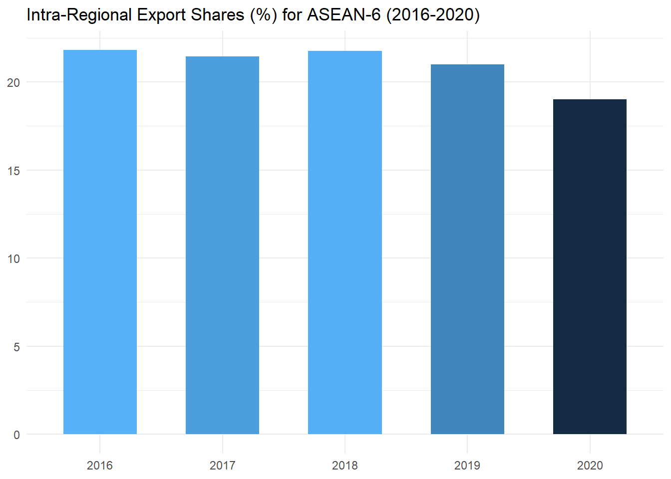

For each year we have calculated the proportion of ASEAN-6’s exports that go to other ASEAN-6 members. This particular export share is called the ASEAN-6 intra-regional export share. The values are visualized in the chart above. As we can see, the intra-regional export share has been decreasing gradually over the examined time period.

3.3 Import Share

What does it tell us? The import share tells us how important a particular trade partner is in terms of the overall import profile of an economy. Changes in the import share over time may indicate that the economies in question are becoming more integrated. In the case of intra-regional import shares, increases in the value over time are sometimes interpreted as an indicator of the significance of a regional trading bloc if one exists, or as a measure of potential if one is proposed.

Definition: The import share is the percentage of imports from the region of interest (the source) to the region under study (the destination) in the total imports of the destination.

Mathematical definition

\(MS = \frac{\sum_{sd} M_{sd}}{\sum_{sw} M_{wd}}\times100\)

where s is the set of countries in the source, d is the set of countries in the destination, w is the set of countries in the world, and M is the bilateral import flow. The numerator is thus imports from the source to the destination, the denominator is total imports to the destination.

Range of values: Takes a value between 0 and 100 per cent, with higher values indicating greater importance of selected trading partner.

Limitations: The intra-regional import share is increasing in the size of the bloc considered by definition, so comparing the shares across different blocs may be misleading. High or low shares and changes over time may reflect numerous factors other than trade policy.

Calculating Import Share follows the same steps as calculating Export Share (as described in the section above). This time we will keep data on import flows in our dataset.

# create a vector with names of ASEAN-6 economies
ASEAN.6 <-  c("Indonesia", "Malaysia", "Philippines", 
              "Singapore", "Thailand", "Viet Nam")

# filter dataset to keep only import flows from ASEAN-6 reporters from ASEAN-6 partners and their total imports from World in 2020
M_ASEAN <- data %>% filter(reporter %in% ASEAN.6 &  year %in% 2020 & 
                             trade_flow == "Import" &
                             partner %in% c(ASEAN.6, "World") & 
                           year == "2020") 

# select variables of interest
MS <- M_ASEAN %>% select(reporter, partner, trade_value_usd, year)

MS

## # A tibble: 38 × 4
##    reporter  partner     trade_value_usd  year
##    <chr>     <chr>                 <dbl> <dbl>
##  1 Indonesia Indonesia          47472333  2020
##  2 Indonesia Malaysia         6933018937  2020
##  3 Indonesia Philippines       592009526  2020
##  4 Indonesia Singapore       12341231341  2020
##  5 Indonesia Thailand         6483756697  2020
##  6 Indonesia Viet Nam         3130605755  2020
##  7 Indonesia World          141568761235  2020
##  8 Malaysia  Indonesia        8729509605  2020
##  9 Malaysia  Malaysia           23476927  2020
## 10 Malaysia  Philippines      2088858852  2020
## # … with 28 more rows

# calculate import share indicators, round the value
MS <- MS %>% summarize(MS = sum(trade_value_usd[partner!="World"]) / 
                         sum(trade_value_usd[partner=="World"])*100)
MS <- round(MS, 2)
MS

## # A tibble: 1 × 1
##      MS
##   <dbl>
## 1  18.9

Now let’s calculate and plot the same indicator for the same regional bloc but for a series of 5 years.

# get the dataset
M_ASEAN <- data %>% filter(reporter %in% ASEAN.6 & 
                             trade_flow == "Import" & 
                             partner %in% c(ASEAN.6, "World") &
                             year %in% 2016:2020) 

ms_plot <- M_ASEAN %>% 
  # group data by year
  group_by(year) %>% 
  # calculate the indicators
  summarize(MS = sum(trade_value_usd[partner != "World"], na.rm= T) / 
              sum(trade_value_usd[partner == "World"], na.rm= T)*100)

ms_plot$year <- as.factor(ms_plot$year)

ms_plot

## # A tibble: 5 × 2
##   year     MS
##   <fct> <dbl>
## 1 2016   20.5
## 2 2017   20.5
## 3 2018   20.2
## 4 2019   19.7
## 5 2020   18.9

# create a bar chart by assigning variables to axes 
MS_plot <- ms_plot %>%   ggplot(aes(x=year, y=MS)) +
  # adding the chart title and removing axis labels
  labs(title = "Intra-Regional Import Shares (%) for ASEAN-6 (2016-2020)", 
       x = NULL, y = NULL) +
  # adding a bar chart to the chart area, specifying the bar width and removing the legend
  geom_bar(aes(fill = MS), stat='identity', width = 0.6, show.legend = F) +
  # applying the minimal theme
  theme_minimal()

MS_plot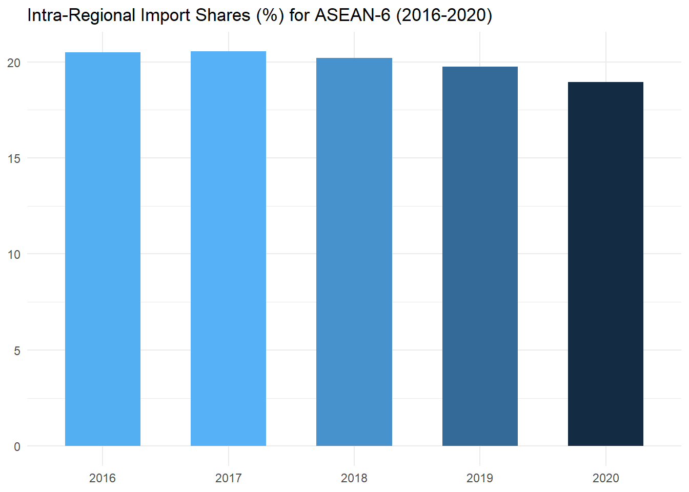

We have now calculated ASEAN-6 intra-regional import shares. The values are plotted in the figure above. As we can see, the intra-regional import share of ASEAN-6 has likewise decreased over the examined period of time.

3.4 Trade Share

What does it tell us? The trade share tells us how important a particular trade partner is in terms of the overall trade profile of an economy. Changes in the trade share over time may indicate that the economies in question are becoming more integrated. In the case of intra-regional shares, increases in the value over time are sometimes interpreted as an indicator of the significance of a regional trading bloc if one exists, or as a measure of potential if one is proposed.

Definition: The trade share is the percentage of the region under study’s trade (imports plus exports) with another region of interest, in the total trade of the region under study.

Mathematical definition

\(TS = \frac{\sum_{sd} X_{sd} + \sum_{ds} M_{ds}}{\sum_{sw} X_{sw} + \sum_{ws} M_{ws}}\times100\)

where s is the set of countries in the source, d is the destination, w is the set of countries in the world, X is the bilateral flow of exports from the source and M is the bilateral import flow to the source. Note the reversal of the usual notation on the import side – we want imports to and exports from the same region when we calculate total trade.

Range of values: Takes a value between 0 and 100 per cent, with higher values indicating greater importance of selected trading partner.

Limitations: The intra-regional trade share is increasing in the size of the bloc considered by definition, so comparing the shares across different blocs may be misleading. High or low shares and changes over time may reflect numerous factors other than trade policy.

To calculate Trade Share indicator for ASEAN-6 we will need to pull together the two datasets used in the sections above and currently stored in objects M_ASEAN and X_ASEAN. After that, we will use spread() to separate Imports and Exports into separate columns. We will also replace any NAs in the datasets with zeros, assuming zero trade flows.

# bind export and import datasets together
TS <- rbind(M_ASEAN, X_ASEAN)

# only keep data on trade flows in 2020, and reshape the data to have export and import flows in separate columns
TS <- TS %>% filter(partner %in% c(ASEAN.6, "World") & year=="2020") %>% 
  spread(trade_flow, trade_value_usd)

# replace any NAs with 0
TS[is.na(TS)] <- 0

TS

## # A tibble: 74 × 6
##     ...1 reporter  partner      year      Export      Import
##    <dbl> <chr>     <chr>       <dbl>       <dbl>       <dbl>
##  1 21254 Indonesia Indonesia    2020           0    47472333
##  2 21302 Indonesia Malaysia     2020  8098764319           0
##  3 21303 Indonesia Malaysia     2020           0  6933018937
##  4 21373 Indonesia Philippines  2020  5900740847           0
##  5 21374 Indonesia Philippines  2020           0   592009526
##  6 21416 Indonesia Singapore    2020 10661853725           0
##  7 21417 Indonesia Singapore    2020           0 12341231341
##  8 21449 Indonesia Thailand     2020  5110298724           0
##  9 21450 Indonesia Thailand     2020           0  6483756697
## 10 21490 Indonesia Viet Nam     2020  4941357726           0
## # … with 64 more rows

In the resulting dataframe please note the presence of rows with matching reporters and exporters and with positive values for import flows. According to this explanation, this is indicative of re-imports where partner attribution is based on country of origin. These data rows can be filtered out, if necessary.

Let’s sum Imports and Exports to get the total trade values between each reporter and partner, and store them in a new column. We can then calculate the Intra-regional Trade Shares and round the values as usual.

# calculate total trade values for each reporter-partner combination
TS$trade_value_usd <- TS$Export + TS$Import

# remove redundant columns
TS <- TS[,c("reporter", "partner", "trade_value_usd")]
TS

## # A tibble: 74 × 3
##    reporter  partner     trade_value_usd
##    <chr>     <chr>                 <dbl>
##  1 Indonesia Indonesia          47472333
##  2 Indonesia Malaysia         8098764319
##  3 Indonesia Malaysia         6933018937
##  4 Indonesia Philippines      5900740847
##  5 Indonesia Philippines       592009526
##  6 Indonesia Singapore       10661853725
##  7 Indonesia Singapore       12341231341
##  8 Indonesia Thailand         5110298724
##  9 Indonesia Thailand         6483756697
## 10 Indonesia Viet Nam         4941357726
## # … with 64 more rows

TS <- TS %>% 
  # calculate intra-regional trade share for ASEAN-6 in 2020, and round the value
  summarize(TS = sum(trade_value_usd[partner!="World"]) / 
              sum(trade_value_usd[partner=="World"])*100)
TS <- round(TS, 2)

TS

## # A tibble: 1 × 1
##      TS
##   <dbl>
## 1  19.0

Now let’s calculate and plot the same indicator for the same regional bloc but for a series of 5 years.

# get the needed dataset
ts_plot <- rbind(X_ASEAN, M_ASEAN)[,c("reporter", "partner", 
                                      "year","trade_value_usd", "trade_flow")]

# filter and reshape the data, fill NAs with 0
ts_plot <- ts_plot  %>% filter(partner %in% c(ASEAN.6, "World")) %>% 
  spread(trade_flow, trade_value_usd)

ts_plot[is.na(ts_plot)] <- 0


ts_plot <- ts_plot %>%  
  # group data by year
  group_by(year) %>% 
  # calculate trade share indicators for each year
  summarize(TS = sum(Export[partner!="World"] + Import[partner!="World"]) / 
              sum(Export[partner=="World"] + Import[partner=="World"])    *100)

ts_plot$year <- as.factor(ts_plot$year)

ts_plot

## # A tibble: 5 × 2
##   year     TS
##   <fct> <dbl>
## 1 2016   21.2
## 2 2017   21.0
## 3 2018   21.0
## 4 2019   20.4
## 5 2020   19.0

# create a bar chart by assigning variables to axes 
TS_plot <- ts_plot %>%   ggplot(aes(x= year, y= TS)) +
    # adding the chart title and removing axis labels
  labs(title = "Intra-Regional Trade Shares (%) for ASEAN-6 (2016-2020)", x = NULL, y = NULL) +
  # adding a bar chart to the chart area, specifying the bar width and removing the legend
  geom_bar(aes(fill = TS), stat='identity', width = 0.6, show.legend = F) +
  # applying the minimal theme
  theme_minimal()

TS_plot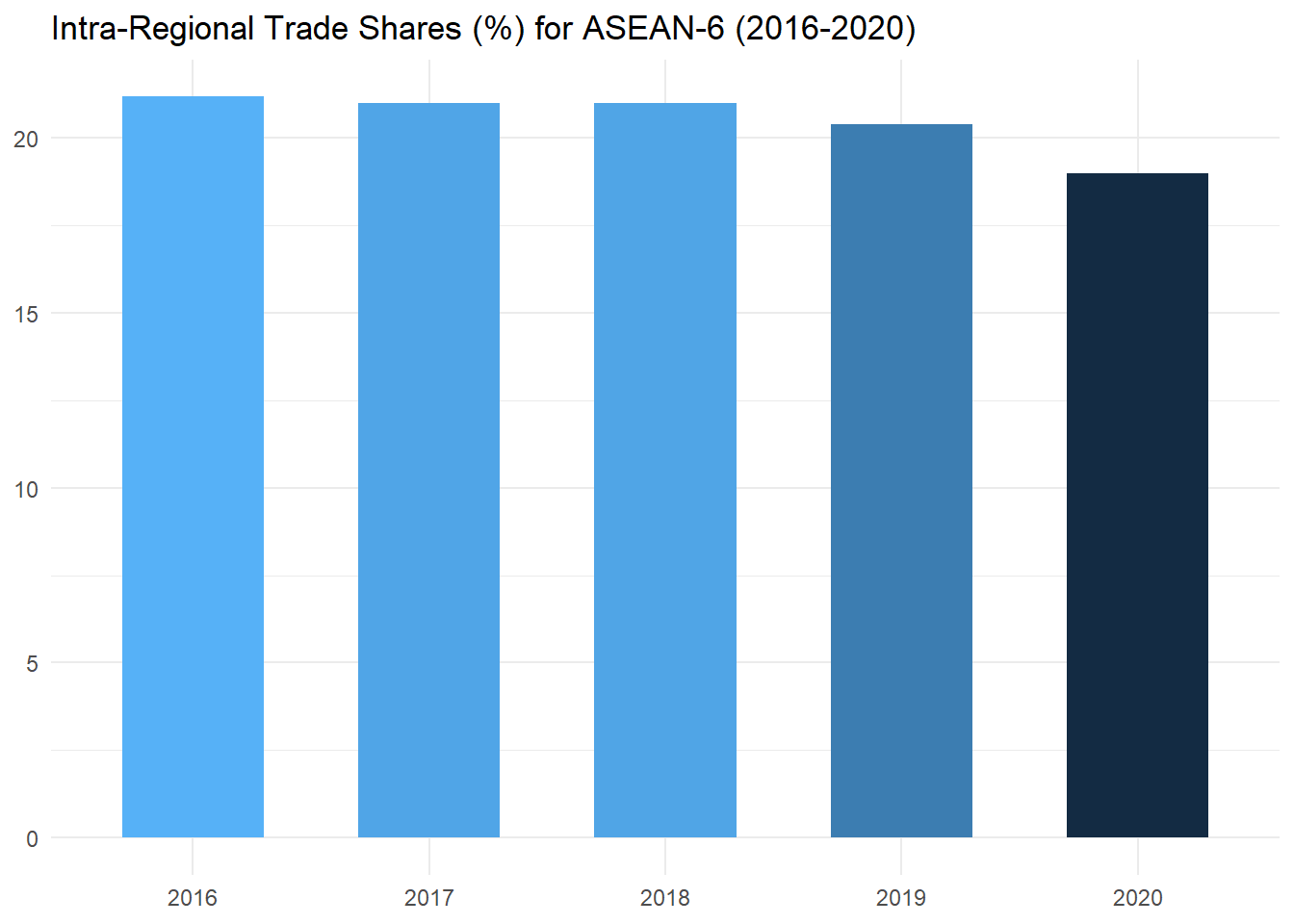

The chart above presents the ASEAN-6 intra-regional trade shares for the years 2016-2020. Given the two preceding examples, it is not surprising that we again observe a gradual decrease in the relative importance of intra-ASEAN-6 trade over time, from around 21 per cent in 2016 to around 19 per cent in 2020. In fact, the intra-regional trade share is a weighted average of the intra-regional export and import shares, with the weights being the share of total imports in total trade and the share of total exports in total trade, and so must lie between the two (see technical notes).

3.5 Regional Market Share

What does it tell us? The regional market share statistic tells us the relative importance of the members of a trade bloc in the intra-regional trade of the bloc. It is a variation on the export share. The larger the value, the more the economy in question dominates the exports of the bloc in question.

Definition: The regional market share is defined as the proportion of total exports of a given member(s) of a trading bloc to other members of the bloc, in the total intra-regional exports of the bloc.

Mathematical definition

\(RMS = \frac{\sum_{sb} X_{sb}}{\sum_{db} X_{db}}\times100\)

where s is the set of source countries under study, b and d are the set of members of the trade bloc under study (the destinations), and X is the bilateral flow of exports from the source to the destination. The elements of s are a subset of b. In words, we have the share of exports from region s to trade bloc b in total intra-regional exports of trade bloc b.

Range of values: Takes a value between 0 and 100 per cent, with higher values indicating greater importance of the economy within the regional trading bloc.

Limitations: The usual limitations of shares apply. A high (or low) regional market share may simply reflect the size of the economy in world trade – i.e., the statistic it not normalized.

For this indicator we need data on exports within the region only, or intra-regional exports. Let’s get back to ASEAN-6 exports dataset and filter to one year, excluding exports to the world. We use group_by() to define total exports from each ASEAN-6 reporter to the bloc and to calculate the shares.

# get the dataset
RMS <- X_ASEAN %>% filter(partner %in% ASEAN.6 & year == 2020)

RMS <- RMS %>% 
  # group by reporter
  group_by(reporter) %>% 
  # calculate regional shares of each reporter in 2020
  summarize(RMS = sum(trade_value_usd) / sum(RMS$trade_value_usd)*100)

# round the values
RMS$RMS <- round(RMS$RMS, 1)

RMS

## # A tibble: 6 × 2
##   reporter      RMS
##   <chr>       <dbl>
## 1 Indonesia    13.5
## 2 Malaysia     24.6
## 3 Philippines   4  
## 4 Singapore    34.6
## 5 Thailand     16.4
## 6 Viet Nam      6.9

We’ll now display regional market shares for each regional economy in a pie chart.

  # create the pie chart by
RMS_plot <- RMS %>% 
  # arranging the data by reporter alphabetically
  arrange(desc(reporter)) %>%
  # calculating position of each sector boundary on the pie chart
  mutate(RMS = round(RMS, 1)) %>% 
  mutate(ypos = cumsum(RMS) - 0.5*RMS) %>% 
  # creating the pie chart
  ggplot(aes(x="", y=RMS, fill=reporter)) +
  geom_bar(stat="identity", width=1, color="white") +
  coord_polar("y", direction = -1) +
  # adding the value labels and title to the chart
  geom_text(aes(x = 1.7, y = ypos, label = paste0(RMS, "%"))) +
  labs(title = "Regional Market Shares for ASEAN-6 (2020)", fill = NULL) +
  # adjusting the aesthetics of the chart
  scale_fill_brewer(palette = "Set1") +
  # applying empty theme
  theme_void()

RMS_plot

The chart above reveals that in 2020 intra-ASEAN-6 exports were heavily dominated by Singapore and Malaysia, which together accounted for nearly 60 per cent of intra-ASEAN-6 trade.

3.6 Trade Intensity

What does it tell us? We can think of the trade intensity index as a uniform export share. In other words, the statistic tells us whether or not a region exports more (as a percentage) to a given destination than the world does on average. It is interpreted in much the same way as an export share. It does not suffer from any ‘size’ bias, so we can compare the statistic across regions, and over time when exports are growing rapidly.

Definition: The trade intensity statistic is the ratio of two export shares. The numerator is the share of the destination of interest in the exports of the region under study. The denominator is the share of the destination of interest in the exports of the world as a whole.

Mathematical definition

\(TI = \frac{\sum_{sd} X_{sd} / \sum_{sw} X_{sw}}{\sum_{wd} X_{wd} / \sum_{wy} X_{wy}}\)

where s is the set of countries in the source, d is the destination, w and y represent the countries in the world, and X is the bilateral flow of total exports. In words, the numerator is the export share of the source region to the destination, the denominator is export share of the world to the destination.

Range of values: Takes a value between 0 and +∞. Values greater than 1 indicate an ‘intense’ trade relationship.

Limitations: As with trade shares, high or low intensity indices and changes over time may reflect numerous factors other than trade policy.

Let’s now calculate Trade Intensity indicators for the economies that are parties to Australia-New Zealand Closer Economic Relations Trade Agreement (ANZCERTA).

Let’s first extract our datasets from data object and make some initial calculations.

# get data on Australia's and New Zealand's exports to each other and to the world in 2020
Xsd_ANZCERTA <- data %>% filter(reporter %in% c("Australia","New Zealand") &
                                  partner %in% c("Australia","New Zealand", "World") &
                                  trade_flow == "Export" & 
                                  year == 2020)
  

# get data on all reporters' exports to Australia and New Zealand in 2020
Xwd_ANZCERTA <- data %>% filter(  partner %in% c("Australia","New Zealand") &
                                  trade_flow == "Export" & 
                                  year == 2020)
  
# use the second dataset to calculate total world exports to Australia and New Zealand
Xwd_ANZCERTA <- Xwd_ANZCERTA %>% group_by(partner) %>% 
  summarize(trade_value_usd = sum(trade_value_usd))

Xwd_ANZCERTA

## # A tibble: 2 × 2
##   partner     trade_value_usd
##   <chr>                 <dbl>
## 1 Australia      192715475372
## 2 New Zealand     33490385924

# get data on all reporters' exports to World in 2020
Xw <- data %>% filter( partner %in% c("World") &
                        trade_flow == "Export" & 
                        year == 2020)


# use the third dataset to calculate total world exports to all partners
Xw <- Xw %>% group_by(partner) %>% 
  summarize(trade_value_usd = sum(trade_value_usd))

Xw

## # A tibble: 1 × 2
##   partner trade_value_usd
##   <chr>             <dbl>
## 1 World           1.71e13

According to the indicator formula, to calculate Trade-Intensity index for ANZCERTA in 2020 we need to take the following steps:

we first need to calculate intra-regional export share for ANZCERTA, i.e. the share of the participating economies’ exports to ANZCERTA region in their total exports to the world;
then we calculate the share of the world’s exports to ANZCERTA region in the total exports of the world;
then we need to find the ratio of the first value to the second value.

In the code chunk below there is a step-by-step calculation option of an indicator, as well as a consolidated calculation option (essentially calculation of in index in one step).

Possibility for a consolidated version will depend of the specific formula and on the data that feeds into it (how much of data pre-processing was done on the dataset before the calculation takes place). However, it is sometimes useful to purposefully break the calculation down into steps, even if a consolidated option is possible. This way it is easier to check the calculation results at each step, which makes it easier to catch a calculation error and to isolate the step where errors exist.

Also note that in this particular case the code for consolidated option is not shorter that the code for a step-by-step calculation

# step-by-step option
TI <- Xsd_ANZCERTA %>%
  # calculate intra-regional export share for ANZCERTA
  summarize(XS_reg = sum(trade_value_usd[partner!="World"])/sum(trade_value_usd[partner=="World"]),
  # calculate share of the world's exports to ANZCERTA region in the total exports of the world
            XS_w = sum(Xwd_ANZCERTA$trade_value_usd)/sum(Xw$trade_value_usd),
  # calculate the trade intensity indicator
             TI = XS_reg / XS_w) %>% select(TI)

# consolidated option
TIx <- Xsd_ANZCERTA %>% 
  summarize(TI = (sum(trade_value_usd[partner!="World"]) /  # intra-ANZCERTA exports
  sum(trade_value_usd[partner=="World"])) /  # total ANZCERTA exports
  (sum(Xwd_ANZCERTA$trade_value_usd) / # world exports to ANZCERTA
      sum(Xw$trade_value_usd))) # World exports to World

# same calculation results
TI == TIx

##        TI
## [1,] TRUE

TI <- round(TI,2)
TI

## # A tibble: 1 × 1
##      TI
##   <dbl>
## 1  3.25

Suppose that we wish to assess the ‘intensity’ of trade among ASEAN-6 economies over a five year period.

Let’s make use of X_ASEAN dataset from one of the previous sections which contains data on export flows to various partners and to the world from ASEAN-6 economies over the examined time period. And let’s use data object to get the rest of the needed datasets as is shown below.

# get data on 2016-2020 exports from all reporters to the first three of the ASEAN-6 economies
Xwd <- data %>% filter( partner %in% ASEAN.6 &
                         trade_flow == "Export" & 
                         year %in% c(2016:2020))
 
# use the dataset to calculate total world exports to ASEAN-6 region in each year
Xwd <- Xwd %>% group_by(year) %>% 
  summarize(Xwd = sum(trade_value_usd))

Xwd

## # A tibble: 5 × 2
##    year           Xwd
##   <dbl>         <dbl>
## 1  2016 1044228578137
## 2  2017 1185831261274
## 3  2018 1305677131579
## 4  2019 1281131875189
## 5  2020 1210134627686

# get data on all reporters' exports to World in 2016-2020
Xw <- data %>% filter( partner %in% "World" &
                         trade_flow == "Export" & 
                         year %in% c(2016:2020))
  
# use the dataset to calculate total world exports to all partners in each year
Xw <- Xw %>% group_by(year) %>% 
  summarize(Xw = sum(trade_value_usd))

Xw

## # A tibble: 5 × 2
##    year      Xw
##   <dbl>   <dbl>
## 1  2016 1.57e13
## 2  2017 1.73e13
## 3  2018 1.89e13
## 4  2019 1.84e13
## 5  2020 1.71e13

# take a look at our vector with ASEAN-6 economy names
ASEAN.6

## [1] "Indonesia"   "Malaysia"    "Philippines" "Singapore"   "Thailand"   
## [6] "Viet Nam"

# filter the ASEAN.6 data frame to remove the redundant data
Xsd <- X_ASEAN %>% filter(partner %in% c(ASEAN.6, "World")) %>%
  group_by(year) %>%
    summarise(
    # calculate total ASEAN-6 export flows to ASEAN-6 region in each year
    Xsd = sum(trade_value_usd[partner!="World"], na.rm = T), 
    # calculate total ASEAN-6 export flows to the World in each year
    Xsw = sum(trade_value_usd[partner=="World"], na.rm = T)
  )

# merge all the the datasets
ti_plot <- left_join(Xsd, Xwd)
ti_plot <- left_join(ti_plot, Xw)

ti_plot

## # A tibble: 5 × 5
##    year          Xsd           Xsw           Xwd      Xw
##   <dbl>        <dbl>         <dbl>         <dbl>   <dbl>
## 1  2016 244315721384 1120266669978 1044228578137 1.57e13
## 2  2017 274503941382 1280252360469 1185831261274 1.73e13
## 3  2018 305728428346 1404341538689 1305677131579 1.89e13
## 4  2019 287195789854 1367438094975 1281131875189 1.84e13
## 5  2020 256552558580 1348969646575 1210134627686 1.71e13

Now let’s make our calculation and then plot the data.

ti_plot <- ti_plot %>%
  # group data by year
  group_by(year) %>%
  # calculate intra-regional export share for ANZCERTA
  summarize(TI = (Xsd/Xsw)/ (Xwd/Xw)) %>% select(year,TI)

ti_plot$year <- as.factor(ti_plot$year)

ti_plot

## # A tibble: 5 × 2
##   year     TI
##   <fct> <dbl>
## 1 2016   3.27
## 2 2017   3.12
## 3 2018   3.16
## 4 2019   3.01
## 5 2020   2.69

# create a bar chart by assigning variables to axes 
TI_plot <- ggplot(ti_plot, aes(x=year, y=TI)) +
  # adding the chart title and removing axis labels
  labs(title = "Trade Intensity Index for ASEAN-6 (2016-2020)", x = NULL, y = NULL) +
  # adding a bar chart to the chart area, specifying the bar width and removing the legend
  geom_bar(aes(fill = TI), stat='identity', width = 0.6, show.legend = F) +                               
  # adding a horizontal line indicating location of 1 on y axis 
  geom_hline(yintercept = 1)+ 
  # applying the minimal theme
  theme_minimal()

TI_plot

The plot above reflects the ‘intensity’ of trade among the economies of ASEAN-6 over a five-year period. Because the index in greater than one, trade within ASEAN-6 during the examined period can be regarded as highly intensive. As is discussed in the handbook, this could be either due to the existence of the trade agreement between the involved economies, or due to their geographic proximity. At the same time intra-regional trade intensity seems to be decreasing over time.

3.7 Size Adjusted Regional Export Share

What does it tell us? The size adjusted regional export share is a variation of the trade intensity index. Its purpose is to normalize the intra-regional export share of a regional trading bloc for group size in world trade. This measure is useful when comparing the intra-regional trade of different trading blocs which vary significantly in terms of the number or level of development of the members. The rationale for the adjustment is that we expect larger groups to have a larger share of world and intra-regional exports.

Definition: The ratio of the intra-regional export share for a given trade bloc, to the share of the bloc’s exports in world trade.

Mathematical definition

\(SAXS = \frac{\sum_{sd} X_{sd} / \sum_{sw} X_{sw}}{\sum_{sw} X_{sw} / \sum_{wy} X_{wy}}\)

where s is the set of countries in the source, d is the destination, w and y the set of countries in the world, and X is the bilateral flow of exports from the source. The numerator is the intra-regional export share of group s. The denominator is the share of group s in world exports.

Range of values: Takes a value between 0 and +∞.

Limitations: As with trade shares, high or low values and changes over time may reflect numerous factors other than trade policy.

Let’s calculate the SAXS indicator for ASEAN-6 in 2020. For this we can reuse the dataset X_ASEAN that we created in one of the sections above. It contains data on export flows to various partners and to the world from ASEAN-6 economies over the examined time period. We will also reuse object Xw which contains data on total world-to-world exports in 2020.

# filter the dataset to keep 2020 export values from from ASEAN-6 economies to ASEAN-6 and to the world
SAXS <- X_ASEAN %>% filter(partner %in% c(ASEAN.6, "World"), year=="2020")
SAXS

## # A tibble: 36 × 6
##     ...1 reporter  partner     trade_value_usd  year trade_flow
##    <dbl> <chr>     <chr>                 <dbl> <dbl> <chr>     
##  1 21302 Indonesia Malaysia         8098764319  2020 Export    
##  2 21373 Indonesia Philippines      5900740847  2020 Export    
##  3 21416 Indonesia Singapore       10661853725  2020 Export    
##  4 21449 Indonesia Thailand         5110298724  2020 Export    
##  5 21490 Indonesia Viet Nam         4941357726  2020 Export    
##  6 21494 Indonesia World          163191837261  2020 Export    
##  7 28447 Malaysia  Indonesia        7039109596  2020 Export    
##  8 28561 Malaysia  Philippines      4188601349  2020 Export    
##  9 28599 Malaysia  Singapore       33816086225  2020 Export    
## 10 28629 Malaysia  Thailand        10786175493  2020 Export    
## # … with 26 more rows

# look at the Xw object which contains data on total world-to-world exports in 2020
Xw

## # A tibble: 5 × 2
##    year      Xw
##   <dbl>   <dbl>
## 1  2016 1.57e13
## 2  2017 1.73e13
## 3  2018 1.89e13
## 4  2019 1.84e13
## 5  2020 1.71e13

# step by step calculation
SAXS1 <- SAXS %>%
  summarise(
    # calculate intra-regional share of ASEAN-6
    XS_reg = sum(trade_value_usd[partner!="World"]) /  sum(trade_value_usd[partner=="World"]), 
    # calculate share of total ASEAN-6 exports in world exports
    XS_reg_world = sum(trade_value_usd[partner=="World"]) / Xw$Xw[Xw$year == 2020],
    # calculate size adjusted regional export share indicator
    SAXS = XS_reg / XS_reg_world
  ) %>% 
  select(SAXS)


# consolidated option
SAXS2 <- SAXS %>% 
  summarize(
    SAXS = (sum(trade_value_usd[partner!="World"]) /  # intra-ASEAN exports
  sum(trade_value_usd[partner=="World"])) /  # total ASEAN exports
(sum(trade_value_usd[partner=="World"]) /
  Xw$Xw[Xw$year == 2020]))  # world exports

# check same indicator values
SAXS1 == SAXS2

##      SAXS
## [1,] TRUE

SAXS <- round(SAXS1, 2)

SAXS

## # A tibble: 1 × 1
##    SAXS
##   <dbl>
## 1  2.41

Now let’s compare values of size adjusted export shares for a few regional blocs on 2020: ASEAN-6, ANZCERTA, APTA, BIMSTEC. For that we can reuse our SAXS index calculation for ASEAN-6, and Xsd_ANZCERTA dataset from one of the sections above. Additionally we will filter our data object to get data on the other two agreements.

# calculate SAXS for ANZCERTA
saXS_ANZCERTA <- Xsd_ANZCERTA %>% 
  summarize(saXS = (sum(trade_value_usd[partner!="World"]) / 
                      sum(trade_value_usd[partner=="World"])) 
            / 
              (sum(trade_value_usd[partner=="World"]) / 
                 Xw$Xw[Xw$year == 2020] ))

saXS_ANZCERTA

## # A tibble: 1 × 1
##    saXS
##   <dbl>
## 1  2.59

# get export data for APTA members
APTA <- c("Bangladesh", "China", "India", "Rep. of Korea", 
          "Lao People's Dem. Rep.", "Sri Lanka", "Mongolia")

# get data on 2020 exports for economies of APTA
Xsd_APTA <-  data %>% filter(reporter %in% APTA &
                                  trade_flow == "Export" & 
                                  year == 2020)


# filter the dataset
Xsd_APTA <- Xsd_APTA %>% filter(partner %in% c(APTA, "World"))

Xsd_APTA

## # A tibble: 39 × 6
##     ...1 reporter partner                trade_value_usd  year trade_flow
##    <dbl> <chr>    <chr>                            <dbl> <dbl> <chr>     
##  1  9088 China    Bangladesh                 15075630650  2020 Export    
##  2  9244 China    India                      66719471588  2020 Export    
##  3  9276 China    Lao People's Dem. Rep.      1491277597  2020 Export    
##  4  9312 China    Mongolia                    1618062436  2020 Export    
##  5  9378 China    Rep. of Korea             112476215948  2020 Export    
##  6  9428 China    Sri Lanka                   3842700338  2020 Export    
##  7  9489 China    World                    2589098353298  2020 Export    
##  8 20659 India    Bangladesh                  7912820501  2020 Export    
##  9 20708 India    China                      19008266696  2020 Export    
## 10 20841 India    Lao People's Dem. Rep.        27873480  2020 Export    
## # … with 29 more rows

# calculate SAXS for APTA
saXS_APTA <- Xsd_APTA %>% 
  summarize(saXS = (sum(trade_value_usd[partner!="World"]) / 
                      sum(trade_value_usd[partner=="World"])) / 
              (sum(trade_value_usd[partner=="World"]) / 
                 Xw$Xw[Xw$year == 2020] ))

saXS_APTA

## # A tibble: 1 × 1
##    saXS
##   <dbl>
## 1 0.578

# get export data for BIMSTEC members
BIMSTEC <- c("Bangladesh", "Bhutan", "India", "Myanmar", 
             "Nepal", "Sri Lanka", "Thailand")

# get data on 2020 exports for the first 4 economies of BIMSTEC
Xsd_BIMSTEC <-  data %>% filter(reporter %in% BIMSTEC &
                                  trade_flow == "Export" & 
                                  year == 2020)

# filter the dataset
Xsd_BIMSTEC <- Xsd_BIMSTEC %>% filter(partner %in% c(BIMSTEC, "World"))

Xsd_BIMSTEC

## # A tibble: 34 × 6
##     ...1 reporter partner    trade_value_usd  year trade_flow
##    <dbl> <chr>    <chr>                <dbl> <dbl> <chr>     
##  1 20659 India    Bangladesh      7912820501  2020 Export    
##  2 20672 India    Bhutan           623079381  2020 Export    
##  3 20886 India    Myanmar          837624324  2020 Export    
##  4 20893 India    Nepal           5854597318  2020 Export    
##  5 20989 India    Sri Lanka       3224131464  2020 Export    
##  6 21005 India    Thailand        3777064249  2020 Export    
##  7 21052 India    World         275488744877  2020 Export    
##  8 31230 Myanmar  Bangladesh        64080147  2020 Export    
##  9 31330 Myanmar  India            695595180  2020 Export    
## 10 31394 Myanmar  Nepal             12896192  2020 Export    
## # … with 24 more rows

# calculate SAXS for BIMSTEC
saXS_BIMSTEC <- Xsd_BIMSTEC %>% 
  summarize(saXS = (sum(trade_value_usd[partner!="World"]) / 
                      sum(trade_value_usd[partner=="World"])) 
            / 
              (sum(trade_value_usd[partner=="World"]) / 
                 Xw$Xw[Xw$year == 2020]))

saXS_BIMSTEC

## # A tibble: 1 × 1
##    saXS
##   <dbl>
## 1  2.27

Combine the calculated indicators into one dataset and create the final plot.

# combine the indicator data
saxs_plot <- data.frame(Trade_Agreement = c("ASEAN", "APTA", "ANZCERTA", "BIMSTEC"),
                        saXS = as.numeric(c(SAXS, saXS_APTA, saXS_ANZCERTA, saXS_BIMSTEC)))
saxs_plot

##   Trade_Agreement      saXS
## 1           ASEAN 2.4100000
## 2            APTA 0.5775225
## 3        ANZCERTA 2.5905068
## 4         BIMSTEC 2.2719406

# create a bar chart by assigning variables to axes, 
# and reordering the agreement names alphabetically
SAXS_plot <- ggplot(saxs_plot, aes(x=saXS, y=reorder(Trade_Agreement, desc(Trade_Agreement)))) +
  # adding the chart title and removing axis labels
  labs(title = "Size Adjusted Regional Export Share (%) for Selected Trade Agreements (2020)", x = NULL, y = NULL) +
  # adding a bar chart to the chart area, specifying the bar width and removing the legend
  geom_bar(aes(fill = saXS),stat='identity', width = 0.6, show.legend = F) +
  # applying the minimal theme
  theme_minimal()

SAXS_plot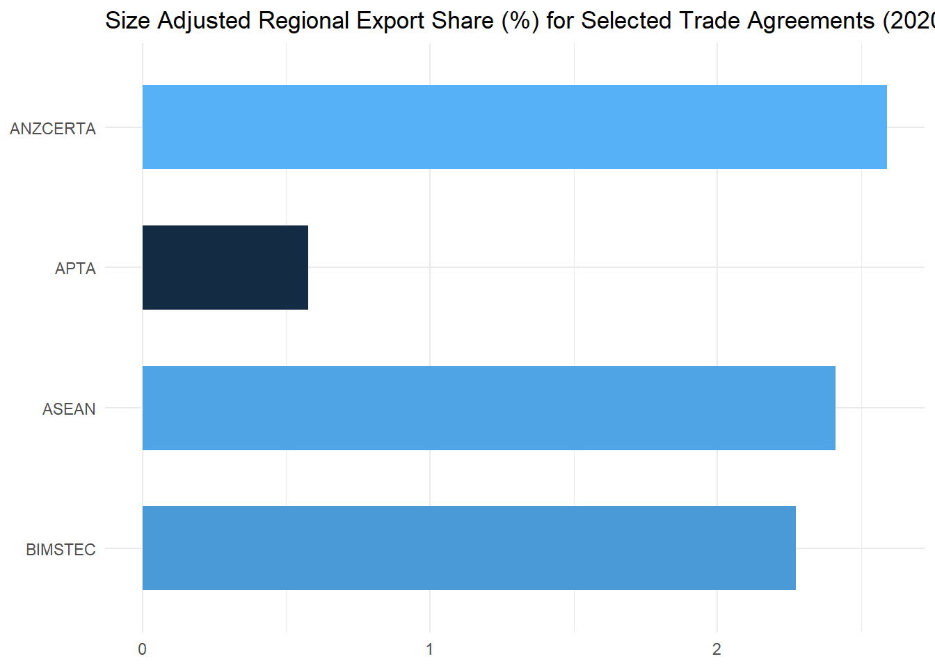

The above figure depicts the size adjusted regional export shares for selected regional trading agreements as of 2020. As we can see, the ANZCERTA has the highest index, which likely reflects geographical proximity of the economies to each other and their geographical isolation from other trading partners. By contrast, the regional bias for APTA is still very low in 2020 (below 1) and is comparable to what was revealed in 2002 as described in the handbook.

3.8 Regional Hirschmann

What does it tell us? The Hirschmann index is a measure of the geographical concentration of exports. It tells us the degree to which a region or country’s exports are dispersed across different destinations. High concentration levels are sometimes interpreted as an indication of vulnerability to economic changes in a small number of export markets. An alternative measure is the trade entropy index.

Definition: The regional Hirschmann index is defined as the square root of the sum across destinations of the squared export shares for the region under study to all destinations.

Mathematical definition

\(RH = \sqrt{\sum_{d}\bigg[\frac{\sum_{s} X_{sd}}{\sum_{sw} X_{sw}}\bigg]^2}\)

where s is the set of source countries under study, d is the set of destinations, w is the set of countries in the world, and X is the bilateral flow of exports from the source to the destination. We want to sum over all destinations, so the sets d and w contain the same elements.

Range of values: Takes a value between 0 and 1. Higher values indicate that exports are concentrated on fewer markets.

Limitations: The Hirschmann index is subject to an aggregation bias – the more disaggregated the data from which it is calculated the better.

Additional notes: A Hirschmann index can also be calculated using import or trade shares. The Hirschmann index is sometimes called the Hirschmann-Herfindahl index (HHI), and is used in other contexts (see the sectoral version later in Chapter 4). It is also calculated in several variants. It may be seen without the final square root operation, or using percentages instead of fractions. It may also be normalized using the number of destinations. The latter adjustment turns the index into a measure of ‘evenness’ in the export share pattern.

Let us now calculate Regional Hirschmann Index (RH) for the Republic of Korea in 2020. First, we obtain the data from UN Comtrade database stored in data object.

Then we calculate export shares to individual partners in the economy’s total exports. After that we square each value (^2) and sum the results up with sum(). Finally we calculate the square root with sqrt()

# retrieve the data on Rep. of Korea's exports to all destinations in 2020
X_KOR <- data %>% filter(reporter %in% c("Rep. of Korea") &
                                  trade_flow == "Export" & 
                                  year == 2020) %>%
  select(reporter, partner, trade_value_usd)
  
X_KOR

## # A tibble: 226 × 3
##    reporter      partner             trade_value_usd
##    <chr>         <chr>                         <dbl>
##  1 Rep. of Korea Afghanistan                29868815
##  2 Rep. of Korea Albania                    22933428
##  3 Rep. of Korea Algeria                   254440961
##  4 Rep. of Korea American Samoa             16232126
##  5 Rep. of Korea Andorra                      271570
##  6 Rep. of Korea Angola                     80161418
##  7 Rep. of Korea Anguilla                     323604
##  8 Rep. of Korea Antarctica                     3323
##  9 Rep. of Korea Antigua and Barbuda         1908543
## 10 Rep. of Korea Areas, nes                 68038381
## # … with 216 more rows

# calculate the RH index
RH <- X_KOR %>% summarize(RH = sqrt(sum((trade_value_usd[partner!="World"] / trade_value_usd[partner=="World"])^2)))
RH <- round(RH, 2)
RH

## # A tibble: 1 × 1
##      RH
##   <dbl>
## 1  0.33

Suppose we wish to understand the change in the degree of geographical dispersion of the exports of the Republic of Korea over a few year period. Let’s first extract get the required set of data.

# retrieve data on Rep. of Korea's exports to all destinations over 2011-2020
X_KOR_plot <- data %>% filter(reporter %in% c("Rep. of Korea") &
                                  trade_flow == "Export" ) %>%
# select variables of interest
  select(reporter, partner, year, trade_value_usd)

X_KOR_plot

## # A tibble: 1,564 × 4
##    reporter      partner              year trade_value_usd
##    <chr>         <chr>               <dbl>           <dbl>
##  1 Rep. of Korea Afghanistan          2020        29868815
##  2 Rep. of Korea Albania              2020        22933428
##  3 Rep. of Korea Algeria              2020       254440961
##  4 Rep. of Korea American Samoa       2020        16232126
##  5 Rep. of Korea Andorra              2020          271570
##  6 Rep. of Korea Angola               2020        80161418
##  7 Rep. of Korea Anguilla             2020          323604
##  8 Rep. of Korea Antarctica           2020            3323
##  9 Rep. of Korea Antigua and Barbuda  2020         1908543
## 10 Rep. of Korea Areas, nes           2020        68038381
## # … with 1,554 more rows

rh_plot  <- X_KOR_plot %>% 
  # group data by year
  group_by(year) %>% 
  # calculate RH index for each year
  summarize(RH = sqrt(sum((trade_value_usd[partner!="World"] / 
                             trade_value_usd[partner=="World"])^2)))

rh_plot

## # A tibble: 7 × 2
##    year    RH
##   <dbl> <dbl>
## 1  2014 0.306
## 2  2015 0.315
## 3  2016 0.312
## 4  2017 0.309
## 5  2018 0.326
## 6  2019 0.318
## 7  2020 0.328

Then we can graph the changes in the Republic of Korea’s RH index over time.

# create a bar chart by assigning variables to axes , 
# and setting year variable to factor
RH_plot <- ggplot(rh_plot, aes(x=factor(year), y=RH)) +
  # adding the chart title and removing axis labels
  labs(title = "Regional Hirschmann Index for Republic of Korea (2014-2020)", 
       x = NULL, y = NULL) +
  # adding a bar chart to the chart area, specifying the bar width and removing the legend
  geom_bar(aes(fill = RH), stat='identity', width = 0.6, show.legend = F) +
  # applying the minimal theme
  theme_minimal()

RH_plot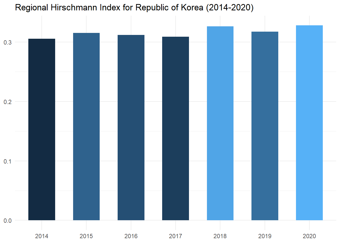

From the chart above we note that over the period of 2011-2020 the index has slightly increased, suggesting that the Republic of Korea has concentrated its export markets on a smaller selection of trade partners.

3.9 Trade Entropy

What does it tell us? The trade entropy index is another measure of the geographical concentration or dispersion of exports. High values indicate that exports are geographically diversified. This can be interpreted as a measure of the degree to which the country under study is integrated with the world economy, or vulnerable to shocks in a limited number of partners.

Definition: The trade entropy index is calculated by summing the export shares multiplied by the natural log of the reciprocal of the export shares (a weight that decreases with the size of the share) of the country under study across all destinations.

Mathematical definition

\(TE = {\sum_{d}\bigg[\frac{\sum_{s} X_{sd}}{\sum_{sw} X_{sw}}\bigg]\ln\bigg[\frac{1}{\sum_{s} X_{sd}/\sum_{sw} X_{sw}}\bigg]}\)

Range of values: Takes a value between 0 and +∞. Higher values indicate greater uniformity in the geographical dispersion of exports. The value of the index is maximized when the export share to every market is the same.

Limitations: The trade entropy index is subject to an aggregation bias.

Let’s now calculate Trade Entropy index for the Rep. of Korea in 2020 using X_KOR dataset from the section on Regional Hirschmann. To take the natural log we use log() function.

TE <- X_KOR %>% 
    summarise(
    # exports shares to each destination
    TE = sum(trade_value_usd[partner!="World"] / trade_value_usd[partner=="World"]  
    #natural log of the reciprocal of the export shares
* log(1/(trade_value_usd[partner!="World"] / trade_value_usd[partner=="World"])))) 

TE <- round(TE, 2)
TE

## # A tibble: 1 × 1
##      TE
##   <dbl>
## 1  3.06

Now let’s calculate TE index for Republic of Korea over a few year period to see the trend over time. We already have all the data from the previous section in X_KOR_plot data frame.

# get the data
te_plot <- X_KOR_plot  %>% 
  # group by year
  group_by(year) %>% 
  # calculate index for each year
  summarize(TE = sum(trade_value_usd[partner!="World"] / 
                       trade_value_usd[partner=="World"] 
                     * 
                       log(1/(trade_value_usd[partner!="World"] / 
                                trade_value_usd[partner=="World"]))))
te_plot

## # A tibble: 7 × 2
##    year    TE
##   <dbl> <dbl>
## 1  2014  3.29
## 2  2015  3.22
## 3  2016  3.21
## 4  2017  3.18
## 5  2018  3.10
## 6  2019  3.13
## 7  2020  3.06

# create a bar chart by assigning variables to axes,
# and setting year variable to factor
TE_plot <- ggplot(te_plot, aes(x=factor(year), y=TE)) +
  # adding the chart title and removing axis labels
  labs(title = "Trade Entropy Index for Republic of Korea (2014-2020)", 
       x = NULL, y = NULL) +
  # adding a bar chart to the chart area, specifying the bar width and removing the legend
  geom_bar(aes(fill = TE),stat='identity', width = 0.6, show.legend = F) +
  # applying the minimal theme
  theme_minimal()

TE_plot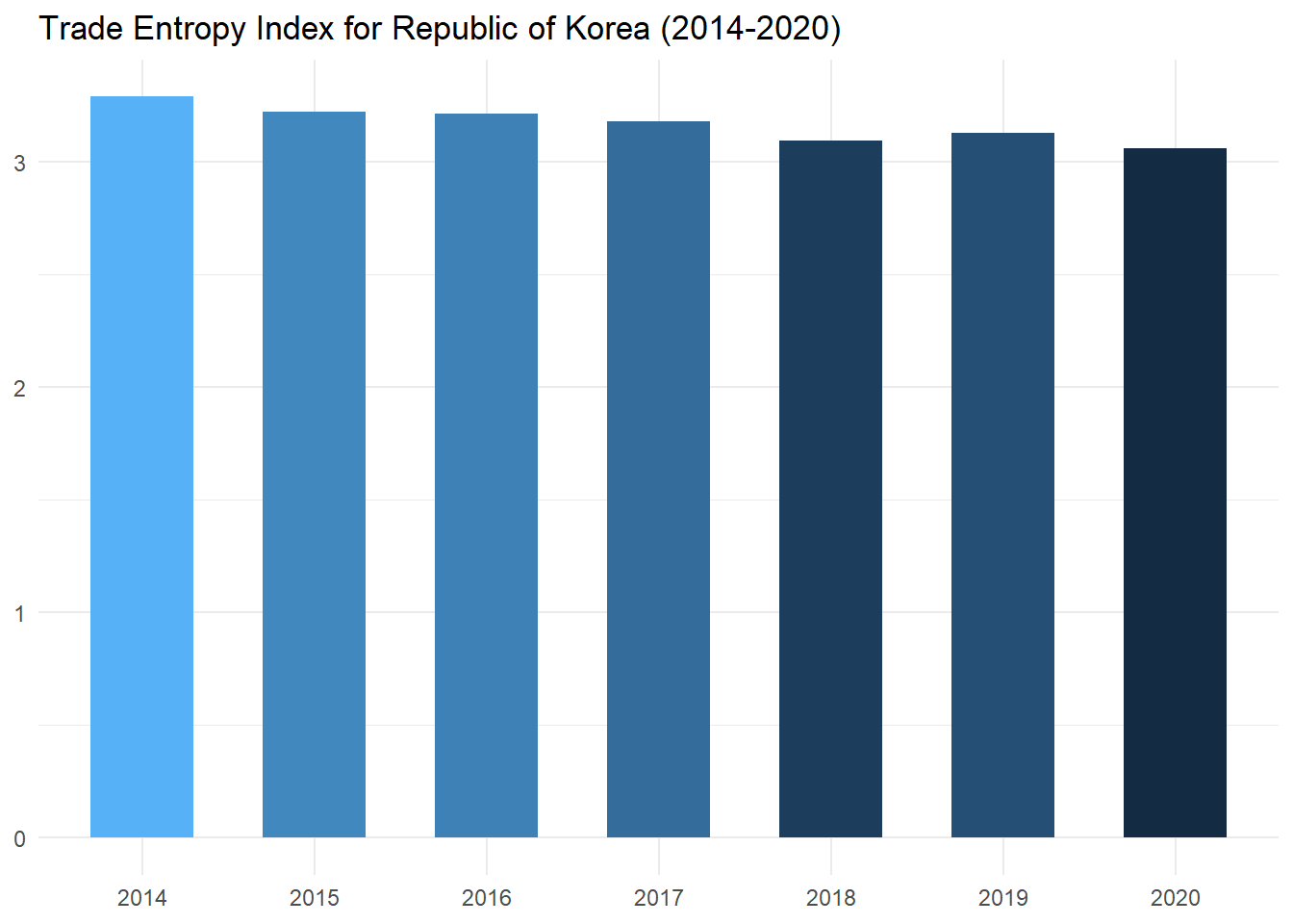

As we compare the trade entropy index with the regional Hirschmann index values for the Rep. of Korea over time, we see that a similar trend of gradually increasing trade partner concentration is revealed in this case as well.