Chapter 8 Regulatory Distance
8.1 Calculating the regulatory distance
In this section we will calculate the regulatory distance between different country-pairs. Regulatory distance is an indicator to measure the similarity between NTM policies across member States. This way we can identify regional trade agreements (RTAs) amongst countries. We calculate the regulatory distance between two countries by summing all the combinations where the two countries have the same product-NTM combination and divide by the total number of product-NTM combinations that exist:
In the formula above \(N\) is the total amount of unique combinations of product codes and NTMs, \(n_{ilk}\) is a dummy variable for country \(i\) applying NTM \(l\) to product \(k\). \(n_{jlk}\) is also a dummy variable, but for country \(j\) applying NTM \(l\) to product \(k\). (For more information on regulatory distance for NTMs, you can check this UNCTAD paper.)
The purpose of this subsection is to create a regulatory distance matrix which will contain all the paired distances between ESCAP countries. To do this, we will complete the following steps:
Step 1: Create the list with ESCAP member countries which have available data.
Step 2: Create an empty regulatory distance matrix, by including ESCAP country ISO3 codes as column and row names.
Step 3: Calculate \(N\) (the total amount of unique combinations of product codes and NTMs).
Step 4: Create a nested for loop to calculate the regulatory distance per country pair.
Let’s first begin by activating the necessary packages we need. There is commented code in case you have not installed them already.
#install.packages("dplyr")
library("dplyr")
#install.packages("readstata13")
library("readstata13")
Next, let’s get the data. In the table below you can find the two data sets we will use. The link to download is in the third column. We will use once again the same NTM data as before In Section 7.
| Description | File name | Link to download |
|---|---|---|
| List of all products which have an NTM | ntm_hs6_2016 v.12.dta | here |
| List of all ESCAP member States | Country Categories.csv | here |
Let’s now load the list of all products which have an NTM. Keep in mind this might take a few minutes.
ntm_data <- read.dta13("data/ntm_hs6_2016 v.12.dta")## Warning in read.dta13("data/ntm_hs6_2016 v.12.dta"):
## notTL:
## Missing factor labels - no labels assigned.
## Set option generate.factors=T to generate labels.Once the data is loaded, we exclude NTM codes which are missing. We only need the reporter, NTM code and product codes (HS 6-digit codes).
ntm_data <- ntm_data[!is.na(ntm_data$ntmcode)&ntm_data$ntmcode!="",]
ntm_data <- ntm_data[,c("reporter", "ntmcode", "hs6")]
We group the data by reporter, NTM and product code (hs6) and count the number of combinations in a new variable called count.
ntm_data <- ntm_data %>% group_by(reporter, ntmcode, hs6) %>%
  summarise(count = n())
head(ntm_data)
## # A tibble: 6 x 4
## # Groups: reporter, ntmcode [1]
## reporter ntmcode hs6 count
## <chr> <chr> <chr> <int>
## 1 AFG A110 010110 1
## 2 AFG A110 010190 1
## 3 AFG A110 010210 1
## 4 AFG A110 010290 2
## 5 AFG A110 010410 1
## 6 AFG A110 010420 1We prepare the regulatory matrix by creating a list of countries for which we want the regulatory distance. Remember the regulatory matrix shows the distance between two countries and has as column and row names the ISO3 codes of the countries.
For the moment we will do this exercise only for ESCAP member States as it is quite time consuming. Readers interested in having the analysis for all available countries are recommended to only run avail_iso3s <- unique(ntm_data$reporter).
We load the file with countries ISO3 codes and select only the ESCAP member States.
countries <- read.csv("data/Country Categories.csv", stringsAsFactors = FALSE)

ESCAP <- countries$iso3[countries$escap==1]
Then we select the unique reporter ISO3 country codes from the NTM data. This list represents all the country codes for which we have available NTM data.
avail_iso3s <- unique(ntm_data$reporter)
head(avail_iso3s)
## [1] "AFG" "ARE" "ARG" "ATG" "AUS" "BEN"We use intersect to find the rows that are both in avail_iso3s and ESCAP. Notice in the final round we have only ESCAP members as expected.
avail_iso3s <- intersect(avail_iso3s,ESCAP)
head(avail_iso3s)
## [1] "AFG" "AUS" "BRN" "CHN" "HKG" "IDN"We create an empty regulatory distance matrix. For column size we use the length of avail_iso3s and add 1 for the reporter column. We populate the column names with reporter and the ISO3 codes with the option dimnames.
regulatory_distance_matrix <- data.frame(matrix(vector(),0,length(avail_iso3s)+1,
                                   dimnames = list(c(), c("reporter", avail_iso3s )
                                   )),
                            stringsAsFactors=F)
Now we can move on to calculating the regulatory distance formula:
As \(N\) is a constant, let’s start with calculating it outside of the loop. Remember, \(N\) is the total number of NTM and product codes combinations in the entire NTM data set. Hence we can use group_by. We define this number under N.
N <- ntm_data %>% group_by(ntmcode, hs6) %>% count()
N <- nrow(N)
We are ready to fill in our regulatory distance matrix with values. In order to do so, we loop through each country in ESCAP and fill in the regulatory_distance_matrix created above. Let’s go through the nested loop together.
We first record all the NTMs (ntmcode) and product codes (hs6) for the first reporter country country_a <- ntm_data[ntm_data$reporter==avail_iso3s[g],c("ntmcode", "hs6")]. We create an additional column where we mark all these combinations with 1: country_a$country_a <- 1. We include the ISO3 country code of the current country under the reporter column: regulatory_distance_matrix[g,"reporter"] <- avail_iso3s[g].
We create a second for statement because we want all possible combinations of country A with the remaining countries. In the second loop, we record all the NTMs (ntmcode) and product codes (hs6) for the second country country_b <- ntm_data[ntm_data$reporter==avail_iso3s[k],c("ntmcode", "hs6")]. We create an additional column where we mark all these combinations with 1 country_b$country_b <- 1. We merge both data sets: merged <- merge(country_a, country_b, by=c("ntmcode", "hs6"), all = TRUE) and include all rows for both data sets. If in the joined data, country A has a combination, which country B doesn’t have - we put a 0: merged[is.na(merged)] <- 0. We create a variable to represent the absolute difference between the indicators for NTMs for both countries: merged$abs_diff <- abs(merged$country_a-merged$country_b). We sum the absolute difference between the two countries and divide the sum by N (the total amount of NTM and product code combinations in the NTM data set): rd <- sum(merged$abs_diff)/N. The resulting value is the regulatory distance rd, which we include in our regulatory distance matrix: regulatory_distance_matrix[g,avail_iso3s[k]] <- rd.
To make this code more efficient, we include the if statement which skips calculating the distance for A and B, if the distance between B and A is already calculated: if (!is.na(regulatory_distance_matrix[k,avail_iso3s[g]])){next }. (This way we end up with a upper triangular matrix.)
Once you are ready, run the codes below. Keep in mind that it might take a few minutes.
for (g in 1:length(avail_iso3s)){
  country_a <- ntm_data[ntm_data$reporter==avail_iso3s[g],c("ntmcode", "hs6")]
  country_a$country_a <- 1
  regulatory_distance_matrix[g,"reporter"] <- avail_iso3s[g]

  for (k in 1:length(avail_iso3s)){

     if (!is.na(regulatory_distance_matrix[k,avail_iso3s[g]])){next }

  country_b <- ntm_data[ntm_data$reporter==avail_iso3s[k],c("ntmcode", "hs6")]
  country_b$country_b <- 1
  merged <- merge(country_a, country_b, by=c("ntmcode", "hs6"), all = TRUE)
  merged[is.na(merged)] <- 0
  merged$abs_diff <- abs(merged$country_a-merged$country_b)
  rd <- sum(merged$abs_diff)/N
  regulatory_distance_matrix[g,avail_iso3s[k]] <- rd

   }
}
Now we fill in the missing values and create a CSV file. For instance, if we have a missing value for country A and country B if (is.na(regulatory_distance_matrix[k,avail_iso3s[g]])), we fill it in with the value from country B and country A regulatory_distance_matrix[k,avail_iso3s[g]] = regulatory_distance_matrix[g,avail_iso3s[k]].
for (g in 1:length(avail_iso3s)){
  for (k in 1:length(avail_iso3s)){
    if (is.na(regulatory_distance_matrix[k,avail_iso3s[g]])){
      regulatory_distance_matrix[k,avail_iso3s[g]] <- regulatory_distance_matrix[g,avail_iso3s[k]]
      }
  }
}

write.csv(regulatory_distance_matrix, "regulatory_distance_matrix_ESCAP.csv")
Quiz
Let’s do a quick practice! Make sure you have run the code on your own.
What is the regulatory distance between Kazakhstan (KAZ) and China (CHN)?
A. 0.12
B. 0.22
C. 0.32
D. 0.02
# You need to run the code and change the path for the "write.csv" command. Once you open it, you can locate that KAZ and CHN have 0.32280137848764 or 0.32 as regulatory distance, hence Answer C is the correct answer. You can find the full table here: https://r.tiid.org/regulatory_distance_matrix_ESCAP.csv8.2 Multidimensional scaling
Using multidimensional scaling (MDS) we can display the information from the regulatory distance matrix by performing principal coordinates analysis. We can therefore show how far or close countries are according to the regulatory distance. This way we can illustrate regional trade agreements (RTAs). Explaining MDS and principal coordinates analysis goes beyond the scope of this guide. As the commands are ready-made and easy to use in R, it is not necessary to have prior knowledge of the methodology. However, readers further interested in MDS and principal coordinates analysis are encouraged to check the help page for the magrittr package for useful references and more information.
First, we download and activate the necessary packages as shown below.
#install.packages("magrittr")
library(magrittr)
##
## Attaching package: 'magrittr'## The following object is masked from 'package:tidyr':
##
## extract#install.packages("dplyr")
library(dplyr)
#install.packages("ggpubr")
library(ggpubr)We first need to render the regulatory distance matrix in the correct format. We copy the regulatory distance matrix and call it regulatory_distance_matrix_MDS. Then we make the row names equal to the reporter column and exclude the reporter column.
regulatory_distance_matrix_MDS <- regulatory_distance_matrix
rownames(regulatory_distance_matrix_MDS) <- regulatory_distance_matrix_MDS$reporter
regulatory_distance_matrix_MDS <- regulatory_distance_matrix_MDS %>% select (-c(reporter))
We perform principal coordinates analysis with the command cmdscale and make a “tibble”. We call the new columns Dim.1 and Dim.2.
regulatory_distance_matrix_MDS <- regulatory_distance_matrix_MDS %>% cmdscale() %>% as_tibble()## Warning: The `x` argument of `as_tibble.matrix()` must have column names if `.name_repair` is omitted as of tibble 2.0.0.
## Using compatibility `.name_repair`.
## This warning is displayed once every 8 hours.
## Call `lifecycle::last_warnings()` to see where this warning was generated.colnames(regulatory_distance_matrix_MDS) <- c("Dim.1", "Dim.2")
head(regulatory_distance_matrix_MDS)## # A tibble: 6 x 2
## Dim.1 Dim.2
## <dbl> <dbl>
## 1 0.0168 0.0158
## 2 -0.0163 -0.00568
## 3 0.0149 0.0111
## 4 -0.271 -0.0340
## 5 0.0159 0.0107
## 6 0.0123 0.0171Dim.1 and Dim.2 represent the countries’ positions on a two-dimensional map such that the distances between the countries are approximately equal to the dissimilarities. The actual values do not mean anything, what is important are the distances between countries.
We can plot this and see the relative distance between countries.
We use ggscatter to plot a scatter plot. We add to our scatter plot a horizontal geom_hline and vertical lines geom_vline to show the horizontal and vertical axis, respectively.
scatterplot <- ggscatter(regulatory_distance_matrix_MDS, x = "Dim.1", y = "Dim.2",
          label = regulatory_distance_matrix$reporter,
          size = 1,
          repel = TRUE)
scatterplot + geom_hline(yintercept=0, linetype="dashed", color = "red") +
  geom_vline(xintercept = 0, linetype="dotted",
                color = "blue")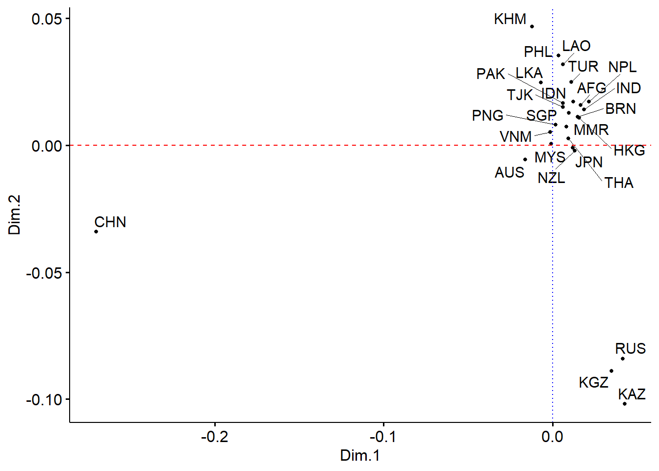
Naturally, most of the ASEAN countries are close to each other (Myanmar, Borneo, Malaysia, Thailand and Singapore). Russia, Kazakhstan and Kyrgyzstan are in the Eurasian Economic Union (EAEU). We can also see that China is quite far away, which is expected as China has one of highest number of NTMs in the world.