Chapter 1 R Basics
1.1 Declaring variables and arithmetics in R
Let’s start with the basic arithmetics like addition, subtraction, multiplication and division.
Let’s first create some variables, in this case “a” and “j” and their values are 34 and 88, respectively. We run this in R:
a <- 34
j <- 88
(Remember you run code by either writing it in the console and pressing “Enter” or by writing a script where you highlight it and press “Control/Command + Enter” or “Command + Enter” for Mac.)
Notice that we use <- to say that “a” is equal to 34.
The equal sign = is the same as the <- operator. It is recommended however to use <-, in order to not confuse = with ==. == is a logical operator (we will use these in Section 2.3) whereas = is for variable or data creation. (There are more reasons why it is advised to use <- when creating variables or data sets. To see the differences between <- and =, {this link}(https://stackoverflow.com/questions/1741820/what-are-the-differences-between-and-assignment-operators-in-r) presents a good discussion.)
a <- 34
a = 34
We can do basic arithmetic operations with our variables, such as addition and division shown below:
a + j## [1] 122a/j## [1] 0.3863636Notice that after each line you see the answer behind ## [1]. For the first code we do not have any output, as we just declare two variables, but as we estimate models or do checks with data sets, without declaring objects, we will get output. Let’s continue, don’t worry this will become clearer as we go further!
Attention! If you happen to run the following code below in the console, R will expect something after the plus. In order to escape this, you need to press the button “Escape”/“Esc”.
a + If we want to access the value of a variable, we can do so by just running its name.
a## [1] 34We can take logarithms with the log command:
log(a)## [1] 3.526361The default logarithm function in R is the natural logarithm.
Quiz
Let’s now practice! Make sure when doing those to have R so if not sure about the correct answer - you can always test it in R! We will not score you on these quizzes, the idea is to train!
What is the correct way to declare a variable called “export” equal to the logarithm of 1000 (log())? (Hint: Look above how we declared a new variable and then combine this with how we take logarithm.)
A. log(1000)
#Answer A is incorrect because it only gives the log value of 1000, but we want to declare the variable export as the logarithm of 1000, therefore the correct answer is C. export <- log(1000). B. export log(1000)
#Answer B is incorrect because it only lists the variable next to the log(1000), however it does not tell R that export is equal to log(1000). In order to tell R that export is equal to log(1000), we must include "<-", therefore the correct answer is C. export <- log(1000). C. export <- log(1000)
#Answer C is correct. Good job! :) 1.2 Class types in R
Variables in R can be of different types, for example a number such as “1011” or character such as “abc”. The type of a variable is referred to as class in R. We check the type of class using the class command. The different types of classes in R have different properties.
The variable a we create is a number and therefore numeric:
a <- 34
class(a)
## [1] "numeric"We check the help file of a function to know what it does with a “?” in front like this:
?Classes_DetailsYou can find all the different classes in R by running the code and scrolling down to “Basic classes”.
Remember the help files can be found on the right of your console.
We would suggest to always have a look at the options a new command has found in its help file. This makes it clear what the new command can do and informs you if you want to change any default settings.
We create a new variable j and put a country name, the class in this case is a “character”.
j <- "China, PRC"
class(j)
## [1] "character"If we wish now to add the two variables a + j, this gives an error now:
a + jError in a + j : non-numeric argument to binary operator
Error messages in R can be very helpful because they indicate why a code is not running and help us build better code. For instance, in the case above, R tells you non-numeric argument to binary operator, which signifies that you cannot mathematically add a “non-numeric” object (in this case j <- "China, PRC"). If you’re uncertain about what the error message means, you can always google it on and add “stackoverflow”.
1.3 Generating distributions
We can get integers from number A to number B such as below:
1:10## [1] 1 2 3 4 5 6 7 8 9 10We can also generate numbers from the random normal distribution with the rnorm command. We can check the help file once again like this:
?rnormRemember to check by yourself the help file of new functions in R. As we go along with this guide, we will explain what new functions do, but for details it is advised to always check the help file.
We can use the above function rnorm to generate 100 numbers with mean of 1 and a standard deviation of 5.
y <- rnorm(100,1,5)We can represent this in a histogram with the hist command.
hist(y)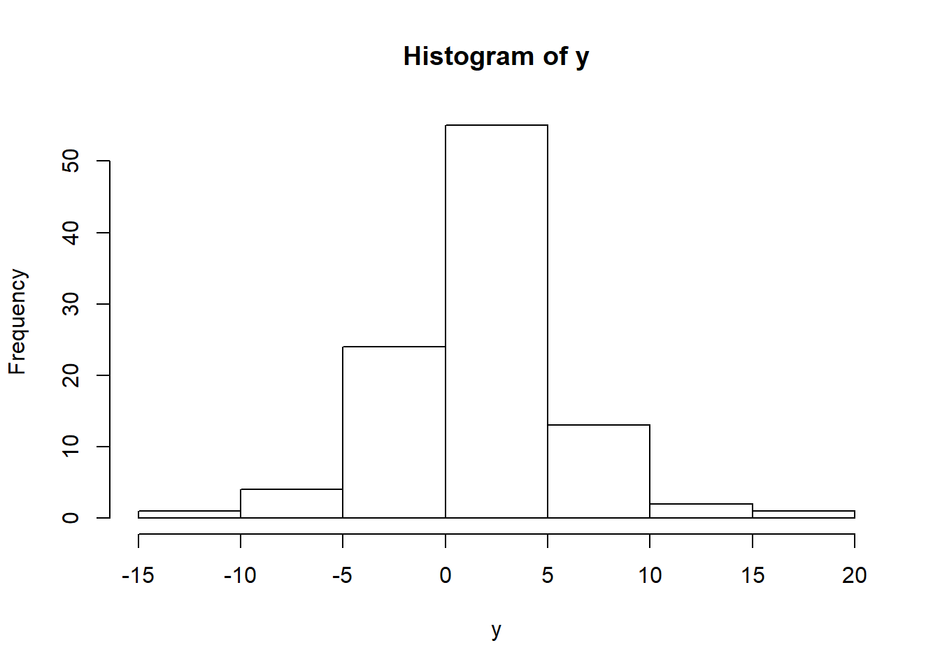
We can create an additional distribution variable “x”, which multiplies “y” by 2 and adds 100 random numbers with mean 0 and a standard deviation of 1.
x <- y * 2 + rnorm(100,0,1)We can visualize the relationship between our two variables “x” and “y” by creating a plot with the plot command. We use the main parameter to add a title, col is for the color of the observations and option 2 is for red.
plot(x,y, main="My first R plot", col=2)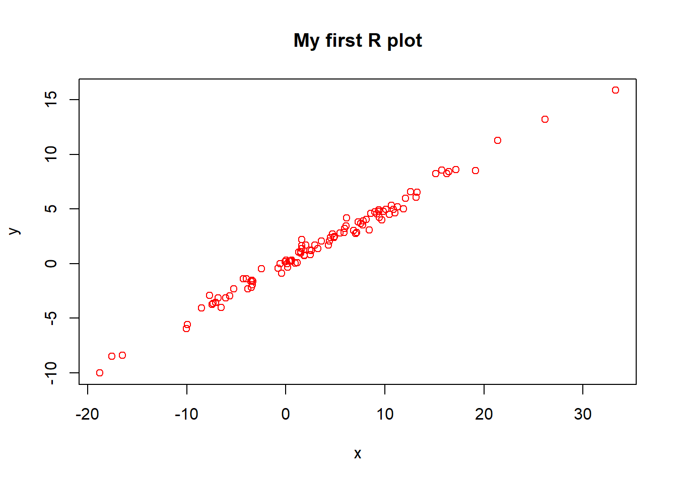
We can also create a prettier colorful plot, worthy of journal submission. By setting col to 1:10, we select all colors with codes from 1 until 10.
plot(x,y, main="My first R plot", col=1:10)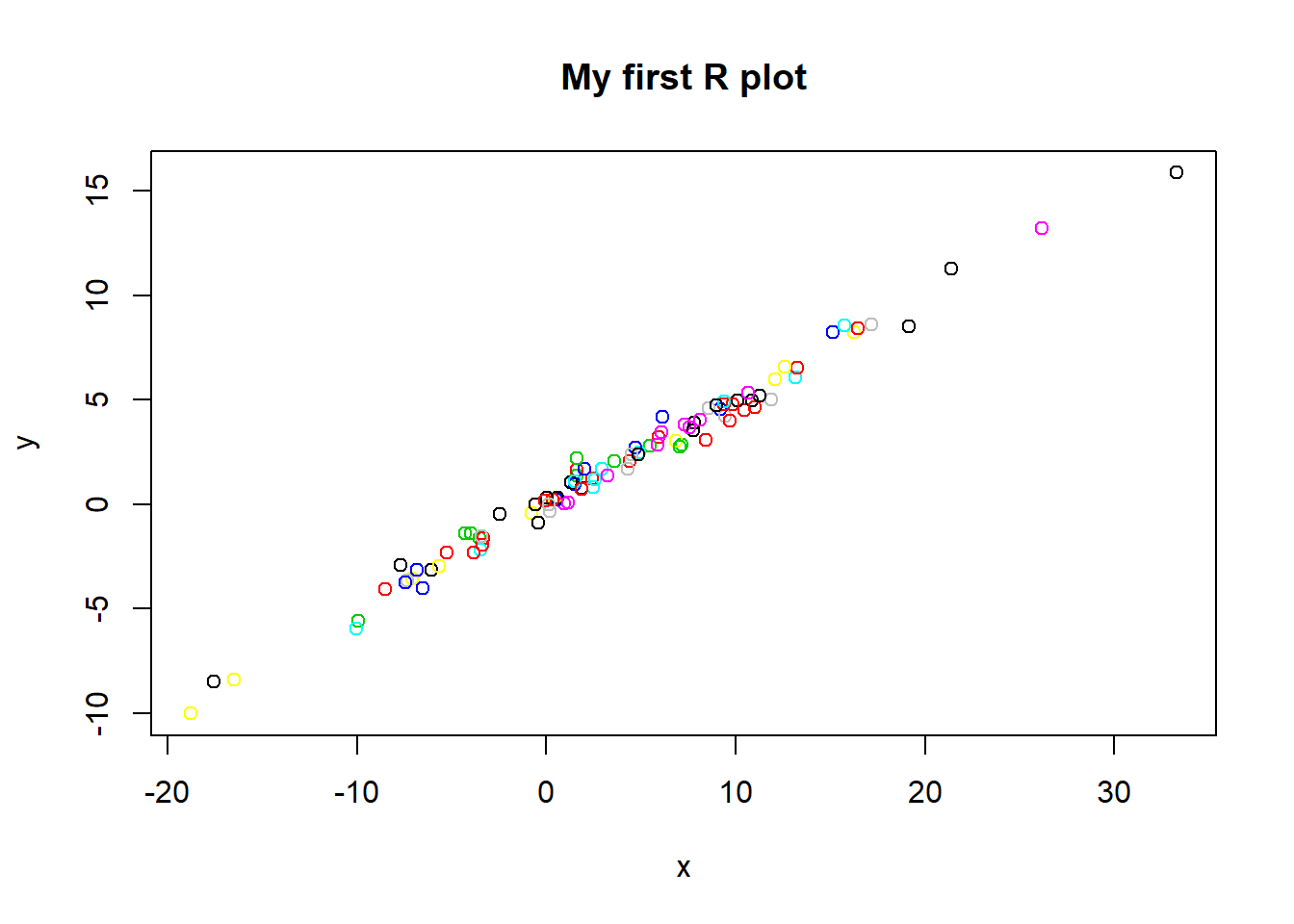
The following plots next are examples with different colors. Note “#000000” is for black.
plot(x,y, col="red")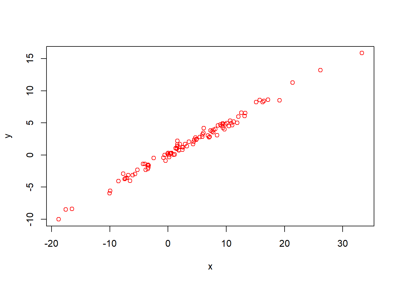
plot(x,y, col="#000000") #black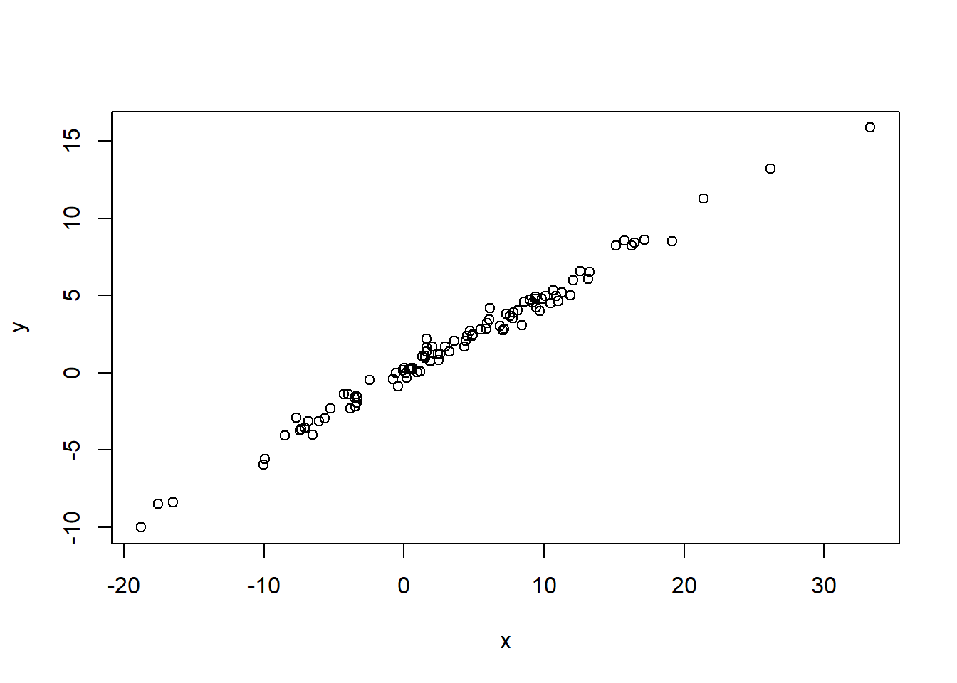
`#black is referred to as a comment. Comments are helpful to give extra explanations or questions. When the computer runs the code, it ignores them. You can make comments by including a “#”.
Quiz
Let’s practice now what we learned so far!
Which answer shows two new variables x and y being generated and a third line plotting them in green with the title “My second R plot!”. (Hint: Check how we did so just now. You can use col=“green”.)
A. x <- rnorm(100,2,5)
y <- x + rnorm(100,1,5)
plot(x,y, main="My second R plot", col="green")
#This is correct. Good job!B. x
y
plot(x,y, main="My second R plot", col="green")
#Answer B is incorrect because it does not specify what x and y should be equal to. The code for the plot is correct though. Therefore the correct answer is A.C. x <- rnorm(100,2,5)
y <- x + rnorm(100,1,5)
plot(x,y)
#Answer C is incorrect because the plot does not specify the title and the points are black, therefore the correct answer is A.