Chapter 6 Non-Tariff Measures (NTMs) and incidence indicators, a simple case
Non-tariff measures (NTMs) are defined as policy measures other than ordinary customs tariffs that can potentially have an economic effect on international trade in goods, changing quantities traded, prices or both. NTMs include technical measures, such as sanitary or environmental protection measures, as well as others traditionally used as instruments of commercial policy, e.g. quotas, price control, exports restrictions, contingent trade protective measures, etc.
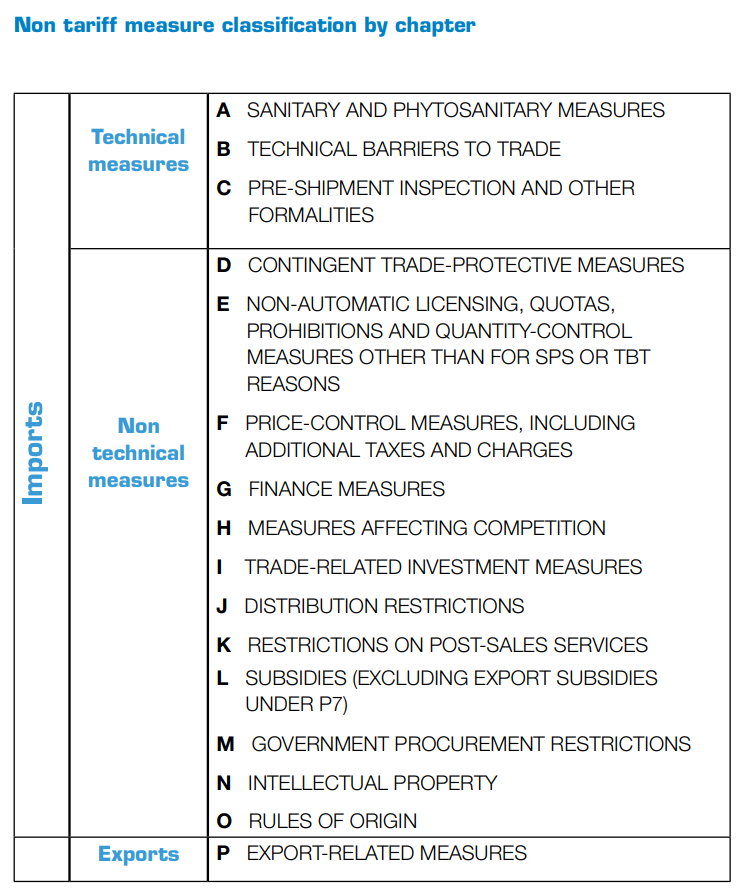
Here you can find UNCTAD’s classification of NTMs (version 2012). The classification of NTMs encompasses 16 chapters (A to P), and each individual chapter is divided into groupings with depth up to four levels. Although a few chapters reach the four-digit level of disaggregation, most of them stop at three digits. For analysis where we have a mixture of three digit levels and four digit levels, we include a zero after the third digit, e.g. “A11” becomes “A110”. All chapters reflect the requirements of the importing country on its imports, with the exception of measures imposed on exports by the exporting country (chapter P). A table with all the chapters is provided below.
The simplest way to study NTMs is to calculate incidence indicators based on the intensity of the policy instruments, and measure the degree of regulation without considering its impact on trade or the economy. Three commonly used incidence indicators are:
- coverage ratio
- frequency index
- prevalence score
These indicators are based upon inventory listing of observed NTMs. The coverage ratio (CR) measures the percentage of trade subject to NTMs, the frequency index (FI) indicates the percentage of products to which NTMs apply, and the prevalence score (PS) is the average number of NTMs applied to products. In this section we will study how to calculate them for all imports and per NTM type.
You can find here UNCTAD’s book where the indicators (coverage ratio, frequency index and prevalence score) are explained on page 92. Data for NTMs can be found here.
(The most recent publication of UNCTAD (2019) presents different options into calculating the NTM indicators. We use the simplest one, but if interested you can find all the alternatives here.)
For now, we will use Lao PDR’s NTM data instead. We use Lao PDR as an example because all imports and NTMs are to the world. This makes the calculations easier since only total imports from trade partners of Lao PDR are required for calculations. For cases when NTMs are applied to only some individual countries or groups, while the same formula is applied - the analysis is a bit more complicated, and is deferred to Section 7 for the case of Viet Nam.
In the table below you can find the two data sets we will use. The link to download is in the third column.
| Description | File name | Link to download |
|---|---|---|
| List of all the products of Lao PDR which have an NTM | lao_ntm.csv | here |
| List of all the imports of Lao PDR | lao_imp.csv | here |
Let’s first load into R the NTM data for Lao PDR. (This is the original source.) This data represents a list of all the products of Lao PDR which have an NTM.
lao_ntm <- read.csv("data/lao_ntm.csv",
                    stringsAsFactors = FALSE)
Let’s download the dplyr package and activate it, if not yet done:
#install.packages("dplyr") #uncomment if not already installed
library("dplyr")
If you get warning (you should), there is a conflict of names for some functions in multiple packages loaded for example:
The following objects are masked from ??package:base??:
intersect, setdiff, setequal, union
In case you need to call a specific function from a specific package, use ::, like this:
base::intersect()dplyr is a very useful and powerful package when performing data processing in R. A very good and intuitive introduction to this package can be found on this link.
The as_data_frame command from dplyr makes a tidy table. By using the following formula, we don’t actually change anything in the data, it simply looks nicer when calling the object by itself.
lao_ntm <- as_data_frame(lao_ntm)## Warning: `as_data_frame()` is deprecated as of tibble 2.0.0.
## Please use `as_tibble()` instead.
## The signature and semantics have changed, see `?as_tibble`.
## This warning is displayed once every 8 hours.
## Call `lifecycle::last_warnings()` to see where this warning was generated.Let’s check how the first few rows look like in Lao PDR’s NTM data. Note because you formatted it with “as_data_frame()” function you don’t need to use “head()” function anymore:
lao_ntm## # A tibble: 27,834 x 5
## reporter partner ntmcode hs6 ntm_1_digit
## <chr> <chr> <chr> <int> <chr>
## 1 LAO WLD A140 10121 A
## 2 LAO WLD A830 10121 A
## 3 LAO WLD A840 10121 A
## 4 LAO WLD C300 10121 C
## 5 LAO WLD F610 10121 F
## 6 LAO WLD F650 10121 F
## 7 LAO WLD P130 10121 P
## 8 LAO WLD P500 10121 P
## 9 LAO WLD P610 10121 P
## 10 LAO WLD P620 10121 P
## # ... with 27,824 more rows(Remember you can open the entire data set by locating the data set name on your right in the section “Environment” and clicking it.)
All the reporter values are LAO and all the partner - WLD for world. As already mentioned Lao PDR’s NTM data contains only the imports from the world. Afterwards we have the four-level codes for NTMs, e.g. A140 which is a special authorization for sanitary and phytosanitary (SPS) reasons and the product code (hs6), e.g. 10121 which is live horses. This tells us that when Lao PDR imports live horses, it needs an authorization. In the final column we have the 1 digit code for NTMs, e.g. A for SPS measures. (HS 6-digit codes or product codes refer to the Harmonized System (HS) for classifying goods in a six-digit format. You can find more about the HS system here.)
Since HS 6-digit codes are product codes and to make the analysis easier to follow, we will use the terms “HS6 code” and “product code” interchangeably everywhere.
Let’s now load in R Lao PDR’s imports:
lao_imp <- read.csv("data/lao_imp.csv", stringsAsFactors = FALSE)Let’s once again have a look at the first rows.
head(lao_imp)## Partner.ISO Commodity.Code Trade.Value..US..
## 1 WLD 10121 1430
## 2 WLD 10190 5100
## 3 WLD 10221 243284
## 4 WLD 10229 32125452
## 5 WLD 10231 22480
## 6 WLD 10239 8630620In this case we have the partner, the Commodity.Code or product code, and the trade value. WLD is the only partner.
unique(lao_imp$Partner.ISO)## [1] "WLD"Let’s rename the variables to something easier to use:
names(lao_imp) <- c("partner","hs6","value")As already mentioned, Lao PDR’s import data is all from the world and therefore unique in product types, as evident also below:
length(unique(lao_imp$hs6))## [1] 3132nrow(lao_imp)## [1] 3132(Notice that the amount of unique product types is the same as the amount of rows, hence all product types mentioned in lao_imp are unique.)
Let’s now use these data sets to calculate the incidence indicators, starting with the coverage ratio.
6.1 Coverage ratio
Let’s begin by calculating the coverage ratio, which shows the percentage trade value subject to NTMs imported by a specific country. The formula for the coverage ratio is as follows:
where \(NTM_{ik}\) is a binary variable, which shows if there is an NTM or not for a traded good \(k\) and \(X_{ik}\) is trade value of good \(k\) for country \(i\).
We have only two terms in this formula for which we need the values - \(NTM_{ik}\) and \(X_{ik}\). We already have the trade value \(X_{ik}\) in the lao_imp data set, so we do not need to do any further calculations for that. For \(NTM_{ik}\) (indicator whether a product imported has an NTM or not), we will extract all the product codes (hs6) from the lao_ntm data. We will count the number of times each product code has an NTM. We will equate \(NTM_{ik}\) to one (\(NTM_{ik} = 1\)) if the count number for NTMs is bigger than 0, otherwise we equate it to 0 (\(NTM_{ik} = 0\)).
Let’s do this step by step.
So we need to get \(NTM_{ik}\), which signifies if a product code has an NTM or not. We first use the lao_ntm data. This summarizes the number of measures for each product (hs6) code:
lao_ntm %>% group_by(hs6) %>% count()## # A tibble: 5,205 x 2
## # Groups: hs6 [5,205]
## hs6 n
## <int> <int>
## 1 10121 10
## 2 10129 13
## 3 10130 13
## 4 10190 13
## 5 10221 10
## 6 10229 13
## 7 10231 10
## 8 10239 13
## 9 10290 13
## 10 10310 10
## # ... with 5,195 more rows% % operators of such type (e.g. %>%) from dplyr are called pipes. %>% says implement this function on the data set. Pipes are considered helpful as they are very easy to use.
So all lao_ntm %>% group_by(hs6) %>% count() does (doesn’t change data, only shows, we do not use <- yet):
1. takes the lao_ntm data set
2. group_by(hs6): groups it by hs6 codes , i.e. multiple rows with the same product code (hs6) are grouped together
3. count(): counts the number of rows where the same product (hs6) code is present
We use the count function in order to sum up all the number of times the same product shows up. Notice that there is no object in between the brackets of count this time. This is because we want to count the last variable mentioned in the pipe, i.e. hs6, so we do not have to refer to it.
Let’s now create a data set:
ntm_hs_freq <- lao_ntm %>% group_by(hs6) %>% count()

head(ntm_hs_freq)
## # A tibble: 6 x 2
## # Groups: hs6 [6]
## hs6 n
## <int> <int>
## 1 10121 10
## 2 10129 13
## 3 10130 13
## 4 10190 13
## 5 10221 10
## 6 10229 13At this stage, ntm_hs_freq is not correct because it has type “P” NTMs or export related measures. (Remember we are interested in Lao PDR’s imports, not the goods it exports, so in this case export related measures to Lao PDR’s exports are not needed.)
We can subset lao_ntm to exclude the “P” measures and count the product codes with count:
ntm_hs_freq <- lao_ntm[lao_ntm$ntm_1_digit!="P",] %>%  #as long as you leave this piple (%>%) last on the line, it will continue to run it acroos multiple lines
  group_by(hs6) %>%
  count()

ntm_hs_freq
## # A tibble: 5,205 x 2
## # Groups: hs6 [5,205]
## hs6 n
## <int> <int>
## 1 10121 6
## 2 10129 9
## 3 10130 9
## 4 10190 9
## 5 10221 6
## 6 10229 9
## 7 10231 6
## 8 10239 9
## 9 10290 9
## 10 10310 6
## # ... with 5,195 more rowsIf you start the line with %>%, the code will not run, but if you end with %>%, it will wait for the next line like an open bracket.
So let’s quickly sum up what we did so far. We created a data set ntm_hs_freq which contains all the product codes which have an NTM in column hs6. Column n contains the number of NTMs applied to a specific product code. Now we need to match these observations to trade values. To do this we merge lao_imp with ntm_hs_freq.
We merge lao_imp with ntm_hs_freq by the product codes. Because the column names match, we can just specify by:
coverage <- merge(lao_imp,ntm_hs_freq,by="hs6",
                  all.x = TRUE)
head(coverage)
## hs6 partner value n
## 1 10121 WLD 1430 6
## 2 10190 WLD 5100 9
## 3 10221 WLD 243284 6
## 4 10229 WLD 32125452 9
## 5 10231 WLD 22480 6
## 6 10239 WLD 8630620 9Adding all.x = TRUE ensures that every row in the lao_imp is kept, otherwise we miss out imports that have zero NTMs.
We will use the columns of the coverage data set to calculate the coverage ratio. Remember for the formula we need the value (\(X_{ik}\)) and the dummy variable \(NTM_{ik}\), signifying whether there is a NTM or not. We will use the number of NTMs n to signify whether there is an NTM or not.
We create a new column called NTMik (\(NTM_{ik}\)) with zeros:
coverage$NTMik <- 0Remember, \(NTM_{ik} = 0\) if no NTMs are found for a product and if at least 1 - \(NTM_{ik} = 1\).
Hence if \(n > 0\), this means at least one NTM is used for that product code, so we change the value of NTMik to 1:
coverage[coverage$n>0,"NTMik"] <- 1In the first part of the formula, we multiply the dummy NTMik by value (or \(X_{ik}\) in the formula):
head(coverage$NTMik*coverage$value)## [1] 1430 5100 243284 32125452 22480 8630620We sum those up:
sum(coverage$NTMik*coverage$value)## [1] 4107068464And divide by the total sum of value (\(X_{ik}\)) then multiply by 100 to get the percentage:
sum(coverage$NTMik*coverage$value)/sum(coverage$value)*100## [1] 100This means that 100% of the imported goods in Lao are subject to NTMs.
Now that you understand the code, let’s go over the steps we took:
1. Define ntm_hs_freq.
2. Merge ntm_hs_freq with lao_imp.
3. Create NTMik.
4. Calculate the formula.
6.1.1 Coverage ratio for SPS measures
Let’s calculate one more coverage ratio to make sure you understand it. Let’s calculate the coverage ratio for SPS (A) measures.
We first define the ntm_hs_freq data. We specify this time that we are only interested in SPS (A) measures, so we change !="P" to =="A":
ntm_hs_freq <- lao_ntm[lao_ntm$ntm_1_digit=="A",] %>%  #as long as you leave this last on the line, it will continue to run it acroos multiple lines
  group_by(hs6) %>%
  count()

ntm_hs_freq
## # A tibble: 1,139 x 2
## # Groups: hs6 [1,139]
## hs6 n
## <int> <int>
## 1 10121 3
## 2 10129 4
## 3 10130 4
## 4 10190 4
## 5 10221 3
## 6 10229 4
## 7 10231 3
## 8 10239 4
## 9 10290 4
## 10 10310 3
## # ... with 1,129 more rows(Small reminder: when we include count(), we tell the R pipe to count on the basis of the last mentioned variable, in this case we use group_by(hs6), therefore we want to count the number of same product codes mentioned.)
We merge lao_imp with ntm_hs_freq using hs6 code just as before:
coverage <- merge(lao_imp,ntm_hs_freq,
                  by="hs6",
                  all.x = TRUE)
head(coverage)
## hs6 partner value n
## 1 10121 WLD 1430 3
## 2 10190 WLD 5100 4
## 3 10221 WLD 243284 3
## 4 10229 WLD 32125452 4
## 5 10231 WLD 22480 3
## 6 10239 WLD 8630620 4Adding all.x = TRUE ensures that every row in the lao_imp is kept, otherwise we miss out imports that have zero SPS measures.
We can create a new column NTMik of zeros, where we will include the NTM dummy variable values.
coverage$NTMik <- 0We change the value of the new variable to 1 if n > 0 meaning a product has at least one SPS measure. This now doesn’t work because we have NA (missing values) because we merged x.all=TRUE before. Hence any NTM that is not an SPS measure (type “A”), has missing values as it is not part of ntm_hs_freq.
coverage[coverage$n>0,"NTMik"] <- 1
Error in [<-.data.frame(*tmp*, coverage$n > 0, "NTMik", value = 1) : missing values are not allowed in subscripted assignments of data frames
So we replace the missing values in “n” with zero by selecting those rows where is.na is true and we only select the “n” column:
coverage[is.na(coverage$n),"n"] <- 0
head(coverage)
## hs6 partner value n NTMik
## 1 10121 WLD 1430 3 0
## 2 10190 WLD 5100 4 0
## 3 10221 WLD 243284 3 0
## 4 10229 WLD 32125452 4 0
## 5 10231 WLD 22480 3 0
## 6 10239 WLD 8630620 4 0So now when we check the n column, there are no rows with missing values:
coverage[is.na(coverage$n), ]## [1] hs6 partner value n NTMik
## <0 rows> (or 0-length row.names)We assign a value of 1 for all \(n > 0\).
coverage[coverage$n>0,"NTMik"] <- 1Now we can calculate the NTM SPS measure once again by summing the product of NTMik multiplied by value (\(X_{ik}\)) and dividing by the total sum of value. We then multiply by 100 to get the percentage!
sum(coverage$NTMik*coverage$value)/
  sum(coverage$value)*100
## [1] 15.57878This number means that 15.6% of trade value that Lao PDR imported had at least one SPS measure.
Quiz
Try now by yourself to calculate the coverage ratio for technical measures. (Hint: the code is similar to above but technical measures belong to Chapter B.)
Which answer is the correct coverage ratio?
(Hint 2: You need to change lao_ntm[lao_ntm$ntm_1_digit=="A",] to lao_ntm[lao_ntm$ntm_1_digit=="B",] in ntm_hs_freq.)
A. 22%
#In order to get the B measures, we need to filter on "ntm_1_digit" and equate it to B. 22% is incorrect because once we run the rest of the code as it is, we get 32%. Hence Answer B is correct!

#Correct code to run:
ntm_hs_freq <- lao_ntm[lao_ntm$ntm_1_digit=="B",] %>%
     group_by(hs6) %>%
     count()

coverage <- merge(lao_imp,ntm_hs_freq,
                  by="hs6",
                  all.x = TRUE)

coverage$NTMik <- 0
coverage[is.na(coverage$n),"n"] <- 0
coverage[coverage$n>0,"NTMik"] <- 1

sum(coverage$NTMik*coverage$value)/sum(coverage$value)*100
## [1] 32.20915B. 32%
#Answer B is correct. Good job! 6.2 Frequency Index
The frequency index is somewhat similar to the coverage ratio, except that we do not multiply with the trade value, but with a dummy signifying whether there is a trade value or not. Hence, the percentage we get shows the share of types of imported goods that are subject to NTMs. The formula is as follows:
where \(NTM_{ik}\) is a binary variable, which shows if there is an NTM or not for a traded good \(k\) and \(D_{ik}\) is also a binary variable showing whether there is any trade value associated with a product \(k\) or not.
We set up the NTM product code frequencies. Once again we exclude export related measures (“P”).
ntm_hs_freq <- lao_ntm[lao_ntm$ntm_1_digit!="P",] %>%
  group_by(hs6) %>%
  count()
In order to get the frequency index, we merge the lao_imp data with ntm_hs_freq.
freq_index <- merge(lao_imp,
                    ntm_hs_freq,
                    by="hs6",
                    all.x = TRUE)
We create a new variable Dik which equals 1 when country \(i\) imports any quantity of product \(k\) and 0 otherwise:
freq_index$Dik <- 0How do we populate this value with 1 if Lao PDR imported anything and zero otherwise?
Dik should be 1 if Lao PDR imported at least 1 dollar.
Let’s start with finding the opposite - all the rows where the value is NA (missing) meaning Lao PDR didn’t import anything:
head(freq_index[is.na(freq_index$value),])## [1] hs6 partner value n Dik
## <0 rows> (or 0-length row.names)To show the rows that are not missing, we write “!” in front is.na:
head(freq_index[!is.na(freq_index$value),])## hs6 partner value n Dik
## 1 10121 WLD 1430 6 0
## 2 10190 WLD 5100 9 0
## 3 10221 WLD 243284 6 0
## 4 10229 WLD 32125452 9 0
## 5 10231 WLD 22480 6 0
## 6 10239 WLD 8630620 9 0We assign 1 only for those with non missing values:
freq_index[!is.na(freq_index$value),"Dik"] <- 1By definition we cannot assign a 1 for missing trade values even if \(n > 0\) because we do not know their values.
Now let’s calculate \(NTM_ik\). Remember NTMik (\(NTM_ik\)) shows us if there is at least one NTM on that product code. Once again we create a new variable called NTMik. We fill it up initially with zeros and set it equal to 1 only if \(n > 0\).
freq_index$NTMik <- 0

freq_index[freq_index$n>0,"NTMik"] <- 1
We divide by the total sum of Dik then multiply by 100.
sum(freq_index$NTMik*freq_index$Dik)/
  sum(freq_index$Dik)*100
## [1] 100This means that 100% of imported products are covered by at least one NTM.
6.2.1 Frequency Index for SPS measures
Next, we calculate the Frequency Index for SPS measures. We first create the ntm_hs_freq data set and merge it with the lao_imp. We create and set Dik to 0.
ntm_hs_freq <- lao_ntm[lao_ntm$ntm_1_digit=="A",] %>%
     group_by(hs6) %>%
     count()

freq_index <- merge(lao_imp,
                    ntm_hs_freq,
                    by="hs6",
                    all.x = TRUE)

freq_index$Dik <- 0
How do we populate this value with 1 if Lao PDR imported something and leave it zero otherwise?
D_ik is 1 if Lao imported at least 1 dollar.
We assign D_ik equal to 1 only for trade values with no missing values:
freq_index[!is.na(freq_index$value),"Dik"] <- 1NTMik shows us if there is at least one NTM on that code. We create and set the value to 0 for NTMik.
freq_index$NTMik <- 0This is different from the above example with the frequency index calculated for all NTMs because some products now have no SPS measures so n (number of NTMs per product code) is missing (NA). Hence we replace the NAs with zero and equate NTMik to 1 only when \(n > 0\).
freq_index[is.na(freq_index$n),"n"] <- 0

freq_index[freq_index$n>0,"NTMik"] <- 1
We calculate the formula.
sum(freq_index$NTMik*freq_index$Dik)/
  sum(freq_index$Dik)*100
## [1] 18.3908Therefore 18.39% of product types face at least 1 SPS measure.
Quiz
Let’s do a quick practice before going to prevalence scores.
What is the frequency index for Lao for NTMs B and C?
A. 31%
B. 54%
C. 12%
D. 17%
#We only need to change the line of the code with which we build the "ntm_hs_freq" data. We change it to:
ntm_hs_freq <- lao_ntm[lao_ntm$ntm_1_digit=="B"|lao_ntm$ntm_1_digit=="C",] %>%
     group_by(hs6) %>%
  count()

#Afterwards, we run everything as it is and it gives us 31.41762 or 31%, which means that Answer A is the correct answer.
freq_index <- merge(lao_imp,
                    ntm_hs_freq,
                    by="hs6",
                    all.x = TRUE)

freq_index$Dik <- 0
freq_index[!is.na(freq_index$value),"Dik"] <- 1
freq_index$NTMik <- 0
freq_index[is.na(freq_index$n),"n"] <- 0
freq_index[freq_index$n>0,"NTMik"] <- 1

sum(freq_index$NTMik*freq_index$Dik)/
  sum(freq_index$Dik)*100
6.3 Prevalence score for SPS measures
The prevalence score (PS) is the average number of NTMs applied to products:
where \(\#NTM_{ik}\) is the number of NTMs per product \(k\) and \(D_{ik}\) is a binary variable showing whether there is any trade value associated with a product \(k\) or not.
We will use the freq_index from the previous section on frequency index as we already have n which is \(\#NTM_{ik}\) and Dik - \(D_{ik}\). Remember, SPS measures are type “A”.
# create NTM product frequencies
ntm_hs_freq <- lao_ntm[lao_ntm$ntm_1_digit=="A",] %>%
     group_by(hs6) %>%
     count()

# merge with imports
freq_index <- merge(lao_imp,
                    ntm_hs_freq,
                    by="hs6",
                    all.x = TRUE)
#create Dik
freq_index$Dik <- 0
freq_index[!is.na(freq_index$value),"Dik"] <- 1

#define missing n as 0
freq_index[is.na(freq_index$n),"n"] <- 0
The formula is as follows:
sum(freq_index$n*freq_index$Dik)/
  sum(freq_index$Dik)
## [1] 0.8125798This means that there are on average 0.8 SPS NTMs applied to imported products in Lao.
Quiz
What is the prevalence score for all types of NTMs (except export related)?
A. 30
B. 20
C. 3.8
D. 1.8
#Once again we can use the frequency index code data, but this time we change the `ntm_hs_freq` to:
ntm_hs_freq <- lao_ntm[lao_ntm$ntm_1_digit!="P",] %>%
     group_by(hs6) %>%
  count()

#We can use the frequency code as before, but use the prevalence formula at the end:
freq_index <- merge(lao_imp,
                    ntm_hs_freq,
                    by="hs6",
                    all.x = TRUE)

freq_index$Dik <- 0
freq_index[!is.na(freq_index$value),"Dik"] <- 1
freq_index$NTMik <- 0
freq_index[is.na(freq_index$n),"n"] <- 0
freq_index[freq_index$n>0,"NTMik"] <- 1


sum(freq_index$n*freq_index$Dik)/sum(freq_index$Dik)

#We get 3.818008 or 3.8, meaning on average imported good in Lao are subject to 3.8 NTMs, hence Answer C is correct.