Chapter 3 More data subsetting and loops in R
3.1 Data subsetting continued
In this section we will dig into more data subsetting and work with the trade_data from the previous section. You will also learn how to make loops!
Once again (if not already done), we load the data here:
trade_data <- read.csv("data/R_tute_data2007-2017.csv")Make sure you are working in your previous directory! You can check this with the command getwd.
We can check the number of rows with nrow.
nrow(trade_data)## [1] 1244330In this case there are 1244330 rows.
An important note is: if you have such big CSV files, do not open with Excel, as Excel’s limit is 1 048 576 rows and the full file will not be loaded. Afterwards when you want to open in R, it will only load the 1 048 576 rows.
Once again we check the variables in this data set:
names(trade_data)## [1] "reporter" "flow" "partner" "year" "value"We can check the first values for a specific column:
head(trade_data$year)## [1] 2008 2008 2008 2008 2008 2008We can also see the unique years in the data set with unique:
unique(trade_data$year)## [1] 2008 2009 2010 2011 2012 2013 2014 2015 2016 2017In the partner column world is “1” and China is “924”.
Let’s find the row that shows the total Chinese exports to the world in 2016:
trade_data[trade_data$flow=="E"& #selects exports
trade_data$reporter==924&        #selects China as reporter
trade_data$year==2016&           #selects the year as 2016
trade_data$partner==1, ]         #selects World as partner
## reporter flow partner year value
## 1019644 924 E 1 2016 2.13659E+12We set global options to get rid of scientific notations by running the following command:
options(scipen = 999)We can make the trade value numeric:
trade_data$value <- as.numeric(as.character(trade_data$value))## Warning: NAs introduced by coercionA warning is issued - that there are missing values now. Depending on the function, some cannot work with missing values, so it is essential to substitute them with estimated values or exclude them. Due to the limited scope of this guide, we will for now ignore the missing values and exclude them. (If interested on this topic, there are methods such as imputation, where if given the correct circumstances we can “impute” or estimate the missing values.)
We can exclude them from our data set in the following way:
trade_data <- trade_data[!is.na(trade_data$value),]Notice how in the above line of code, we first specify our data set, because this is what we want to change and then we specify the command is.na onto the variable value. is.na checks if there are missing values. We include in front of is.na a !, which means that we exclude the missing values.
We can now check the value in billion by dividing the previous function by a billion. Notice after the comma we specify the value column.
trade_data[trade_data$flow=="E"&
trade_data$reporter==924&
trade_data$year==2016&
trade_data$partner==1,"value"
]/1000000000
## [1] 2136.59We can also sum up all the Chinese exports values that are not to the world to see if the total number matches the number above (2136.59). We first need to subset the data to not include the world. We can do so by making the partner not equal != to the world.
head(trade_data[trade_data$flow=="E"&
trade_data$reporter==924&
trade_data$year==2016&
trade_data$partner!=1,
])
## reporter flow partner year value
## 1016163 924 E 293 2016 6081495000
## 1016164 924 E 672 2016 1236859000
## 1016166 924 E 744 2016 1320129000
## 1016184 924 E 399 2016 217025000
## 1016193 924 E 156 2016 27854748000
## 1016255 924 E 405 2016 102783000000Using this we can create a subset data with export values in billion:
CN_X_2016<-trade_data[trade_data$flow=="E"&
trade_data$reporter==924&
trade_data$year==2016&
trade_data$partner!=1,
"value" #added value because that's what we're interested in
]
sum(CN_X_2016)/1000000000
## [1] 8012.502We can notice this number is greater than what we got above (2136.59). This is because the value for China includes economic regions and hence country values are summed twice or more. In order to know which code is for a single country or an economic region, we can use IMF’s data dictionary. Click here to download.
codes <- read.csv("data/imf_codes.csv")
head(codes)
## code iso2 country isCountry region
## 1 110 XR29 Advanced Economies (IMF) 0
## 2 512 AF Afghanistan 1 Asia Pacific
## 3 605 F1 Africa 0
## 4 799 F19 Africa not specified 1 Africa and Middle East
## 5 914 AL Albania 1 Europe
## 6 612 DZ Algeria 1 Africa and Middle East
## income_level AP_region LLDC LDC SIDS
## 1 NA NA NA
## 2 low_income South and South-West Asia 1 1 0
## 3 NA NA NA
## 4 0 0 0
## 5 upper_middle_income 0 0 0
## 6 upper_middle_income 0 0 0In this case we need only the columns: code, country, isCountry, region.
We can overwrite the original codes data frame with only those columns:
codes <- codes[, c("country","code", "isCountry", "region" )]We can also change the order:
codes <- codes[, c("code","country", "isCountry", "region" )]Now, let’s change trade_data so it only includes countries and no economic regions.
How can we do so? There is a column called isCountry which if equal to 1 signifies that the code belongs to a country. We also would like to have world trade values. How can we add now those two conditions?
- First we filter:
codes$isCountry==1by selecting only rows whereisCountry==1.
- Then we add the “or” condition (
|) where we select rows withcodecolumn equal to 1.
- After the comma, we select only the
codecolumn from the data frame. (If left empty, we will get the whole data set - try it!codes[codes$isCountry==1|codes$code==1,])
We use this and create a new data subset of the data set codes:
cntry_w <- codes[codes$isCountry==1|codes$code==1,"code"]So cntry_w is a list of IMF codes that are real countries (not aggregates like advanced economies) as well as 1 to represent world total.
We can use this data set to expand the filters of CN_X_2016 and compose a data set of only Chinese exports to countries and the world in 2016. We do so by specifying trade_data$partner %in% cntry_w, meaning we take country codes only from cntry_w.
CN_X_2016<-trade_data[trade_data$flow=="E"& #select only exports
trade_data$reporter==924& #from china
trade_data$year==2016& #in 2016
trade_data$partner!=1& #where country is not world (code for world is 1)
trade_data$partner %in% cntry_w, #which is in the list of codes that we filtered earlier
"value" #variable we're interested in
]
sum(CN_X_2016)/1000000000
## [1] 2135.245Now we get 2135.25 which is closer to 2136.59, than 8012.50. The difference is due world regions which are not specified as countries.
Quiz
Time for a quick recap! Don’t forget to run the codes in R to check.
What is the correct line of code to select all the exports from China (924) to the world (1) for 2016? (Hint: Look at what we did previously for 2016.)
A. trade_data[trade_data$reporter==924&
trade_data$year==2016&
trade_data$partner==1,
"value"]
#Answer A is incorrect because we did not filter on exports (`trade_data$flow="E"&`). Answer D includes this, hence it is the correct answer. B. trade_data[trade_data$flow="E"&
trade_data$reporter=924&
trade_data$year=2016&
trade_data$partner=1,
"value"]
#Answer B is incorrect because we use "=" instead of "==". Remember "==" is for checking values whereas "=" is for declaring them. (For example trade = 100 declares a new variable trade with value 100, but trade == 1000, checks whether the already existing variable trade is of value 1000.) Hence, Answer D is the correct answer. C. trade_data[flow=="E"&
reporter==924&
year==2016&
partner==1,
"value"]
#Answer C is incorrect because the column variables of our dataset are not objects in R, therefore R cannot find them just by name - we have to specify they are from the trade_data dataset - e.g. trade_data$flow. Hence Answer D is correct.D. trade_data[trade_data$flow=="E"&
trade_data$reporter==924&
trade_data$year==2016&
trade_data$partner==1,
"value"]
#Answer D is correct. Good job! :). 3.2 Creating plots
Now let’s try to plot only the year and value from the Chinese exports data set.
First, we create a data set containing China’s total exports to the world (1) for all years available:
CN_X <- trade_data[trade_data$flow=="E"&
trade_data$reporter==924&
trade_data$partner==1,
]
head(CN_X)
## reporter flow partner year value
## 24180 924 E 1 2008 1428870000000
## 148613 924 E 1 2009 1202050000000
## 273046 924 E 1 2010 1578440000000
## 397479 924 E 1 2011 1899280000000
## 521912 924 E 1 2012 2050090000000
## 646345 924 E 1 2013 2210660000000We can use the plot command to show China’s exports to the world per year:
plot(CN_X[,c("year", "value")])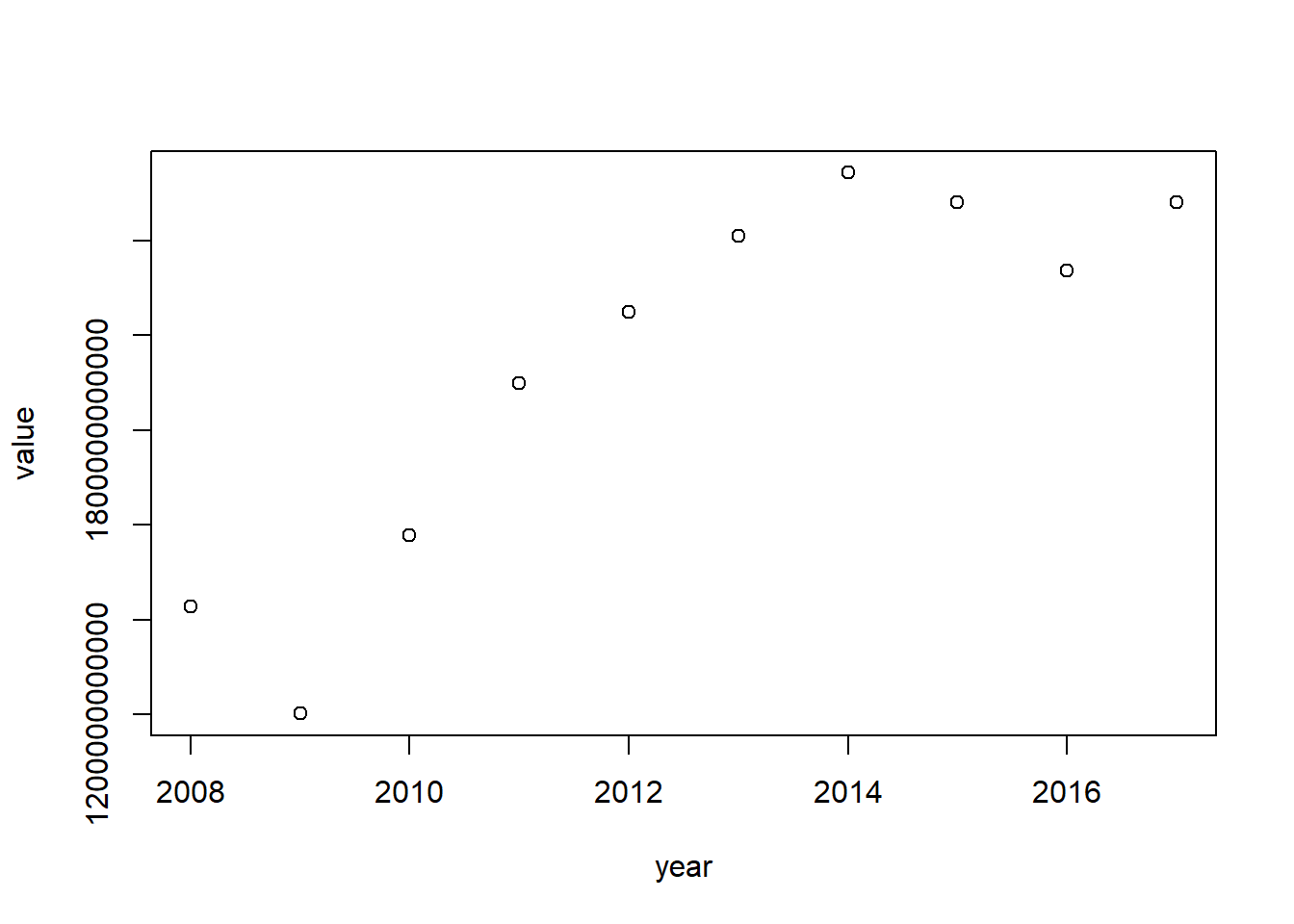
Change the values into trillions:
CN_X$value <- CN_X$value/1000000000000Looks better now:
plot(CN_X[,c("year", "value")])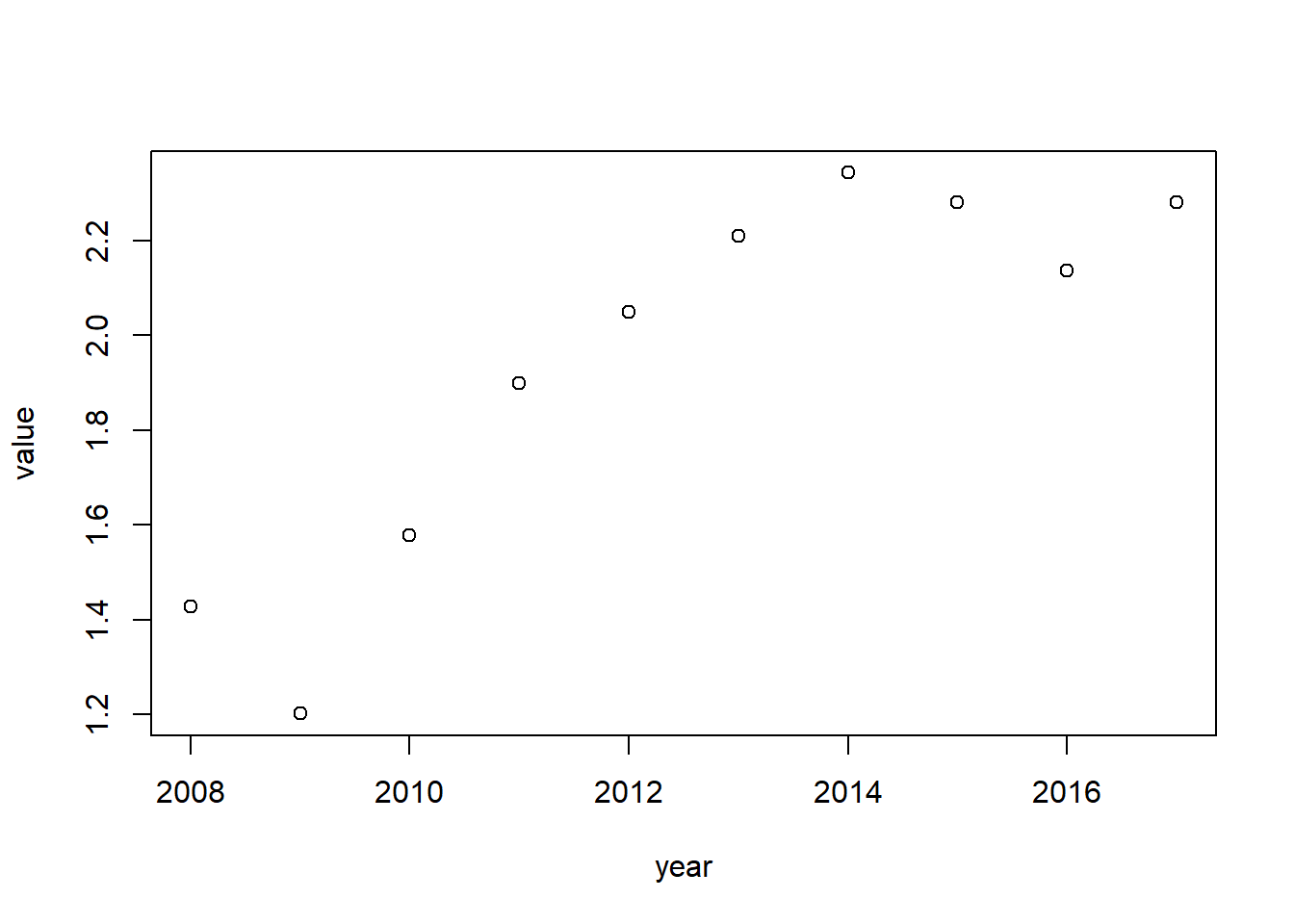
Let’s add a title and y-axis title:
plot(CN_X[,c("year", "value")],
main="China's exports",
xlab="",
ylab="USD, trillions")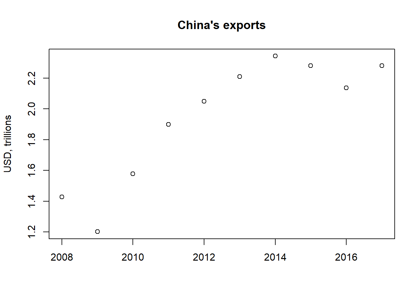
Notice, we use the main command to add a title. xlab and ylab are used for naming the x and y axis respectively.
Points don’t make sense, let’s use a line instead:
plot(CN_X[,c("year", "value")],
main="China's exports",
xlab="",
ylab="USD, trillions",
type="l") #type line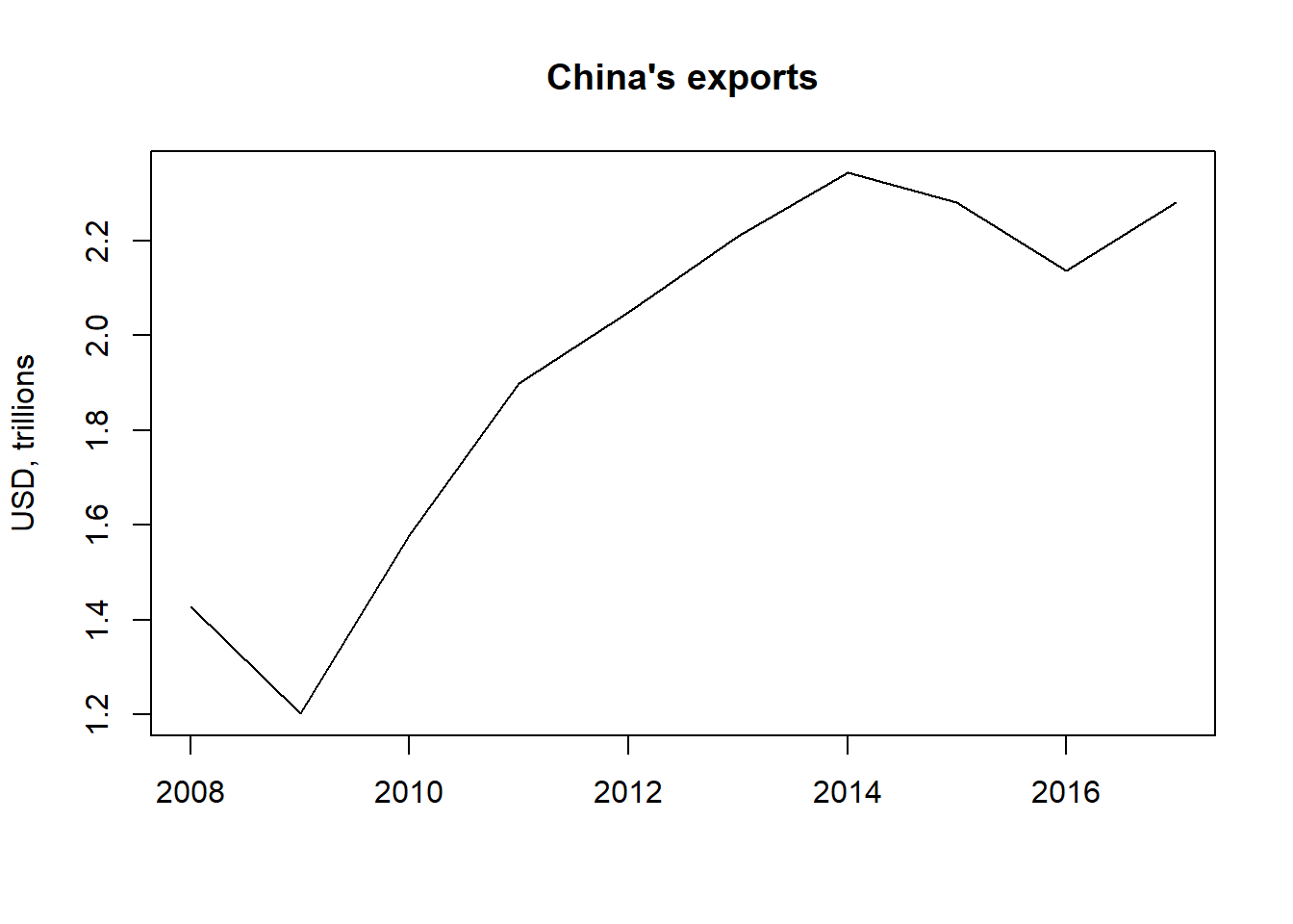
We use a line by setting type = l (“l” as in line, not a 1), the default is p for points. (You can check ?plot for details.)
We can also look at China’s imports and plot this alongside with a legend. Have a look at the code first, the explanation is below.
CN_M <- trade_data[trade_data$flow=="I"&
trade_data$reporter==924&
trade_data$partner==1,
]
CN_M$value <- CN_M$value/1000000000000


plot(CN_X[,c("year", "value")],
main="China's exports and imports",
xlab="",
ylab="USD, trillions",
type="l",
ylim=c(1,2.5), #adding y axis limits
col=2, #red color
lty=1 #solid line, see ?par for details
)
lines(CN_M[,c("year", "value")],col=4, lty=2) #blue color, dashed line

legend("bottomleft",
legend = c("Exports", "Imports"),
col=c(2,4),
lty=c(1,2)
)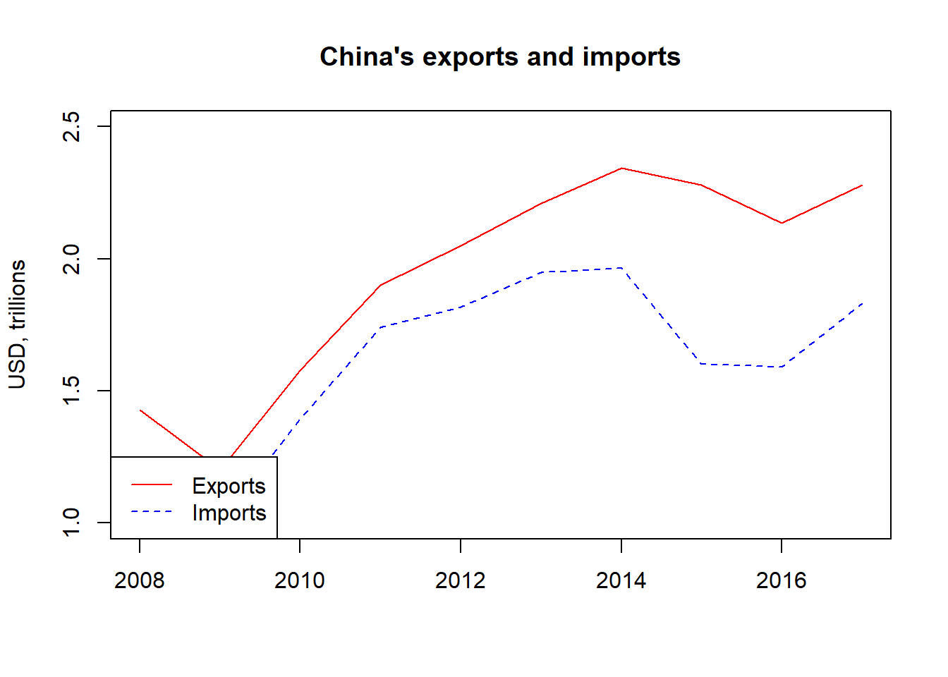
We first create the data set for Chinese imports CN_M. We filter the trade_data by selecting only imports: trade_data$flow=="I", the reporter as China: trade_data$reporter==924 and the partner as the world: trade_data$partner==1. We put the values of this data set in trillions: CN_M$value <- CN_M$value/1000000000000.
We combine both exports CN_X and imports CN_M into one plot by specifying the options for the first line and afterwards specifying lines() which adds a second line. We specify first the plot for CN_X and select the variables years and trade value: CN_X[,c("year", "value")]. We include a title main="China's exports and imports" and a y-axis label ylab="USD, trillions". We specify that we want a line type="l". We can tell R what coordinate system to use for the x-axis and y-axis, with xlim and ylim, respectively. We specify the color with col and a solid line with lty=1. ?par contains all the plot options available. (?plot will also provide you with some options, but the full list is available in par.)
For the second line we specify the data set variables to be used: CN_M[,c("year", "value")], we make the line blue: col=4 and dashed: lty=2.
We add a legend with the command legend. We specify where in our plot we want the legend (e.g. bottom left in this case), provide the names of the items in the legend: legend = c("Exports", "Imports") and include the same specifications from the plot function for the colors: col=c(2,4) and the type of the line: lty=c(1,2). Notice we join the all of the listed specifications with c, as we want them to appear together. In Section 4, we will delve more into plots.
Let’s now show in a plot the top 10 countries China exported to in 2016.
We start by creating a table with Chinese exports in 2016 to individual countries:
CN_X_countries <-
trade_data[trade_data$flow=="E"&
trade_data$reporter==924&
trade_data$year==2016&
trade_data$partner!=1,]

head(CN_X_countries)
## reporter flow partner year value
## 1016163 924 E 293 2016 6081495000
## 1016164 924 E 672 2016 1236859000
## 1016166 924 E 744 2016 1320129000
## 1016184 924 E 399 2016 217025000
## 1016193 924 E 156 2016 27854748000
## 1016255 924 E 405 2016 102783000000We want to have the names of the countries in our plot. To do this, we merge the CN_x_countries data with the codes data by using the merge command.
CNX_merged <- merge(CN_X_countries,
codes, by.x="partner",
by.y="code")
CNX_merged <- CNX_merged[, c("country", "value", "isCountry","region")]

head(CNX_merged)
## country value isCountry region
## 1 Export earnings: fuel 167185000000 0
## 2 Export earnings: nonfuel 1969410000000 0
## 3 Advanced Economies (IMF) 1403500000000 0
## 4 United States 389714000000 1 North America
## 5 United Kingdom 56645733000 1 Europe
## 6 Austria 2245591000 1 EuropeTo use the merge command we first specify the data sets we want to merge - in this case CN_X_countries with codes. We specify the names of the columns by which the data sets should be merged, since they have different names but essentially contain the same factor/categorical data. by.x is for the first data set and by.y - for the second. (If the two data sets had the same name, we do not need to specify by, by.x or by.y.)
Finally, we only keep the variables country, value, isCountry, region. isCountry we use to exclude non-countries and region - to use the same color for the same regions.
We exclude non-countries:
CNX_merged <- CNX_merged[CNX_merged$isCountry==1,]We sort the data with the order command. This sorts the data frame based on value in ascending order:
CNX_merged <- CNX_merged[order(CNX_merged$value),]
head(CNX_merged)
## country value isCountry region
## 65 Montserrat 110000 1 Latin America and Carribean
## 60 Greenland 993000 1 North America
## 11 San Marino 1506000 1 Europe
## 178 Nauru 1644000 1 Asia Pacific
## 174 Faroe Islands 1737000 1 Europe
## 68 St. Kitts and Nevis 4850000 1 Latin America and CarribeanThis sorts the data in descending order:
CNX_merged <- CNX_merged[order(-CNX_merged$value),]
head(CNX_merged)
## country value isCountry region
## 4 United States 389714000000 1 North America
## 101 Hong Kong, China 293997000000 1 Asia Pacific
## 19 Japan 129617000000 1 Asia Pacific
## 105 Korea, Republic of 95815599000 1 Asia Pacific
## 10 Germany 66044117000 1 Europe
## 116 Viet Nam 62040928000 1 Asia PacificWe subset the top 10 export countries in CNX_merged_top10. We illustrate the data with a pie chart with the pie command.
CNX_merged_top10 <- head(CNX_merged,10)

pie(CNX_merged_top10$value,
CNX_merged_top10$country)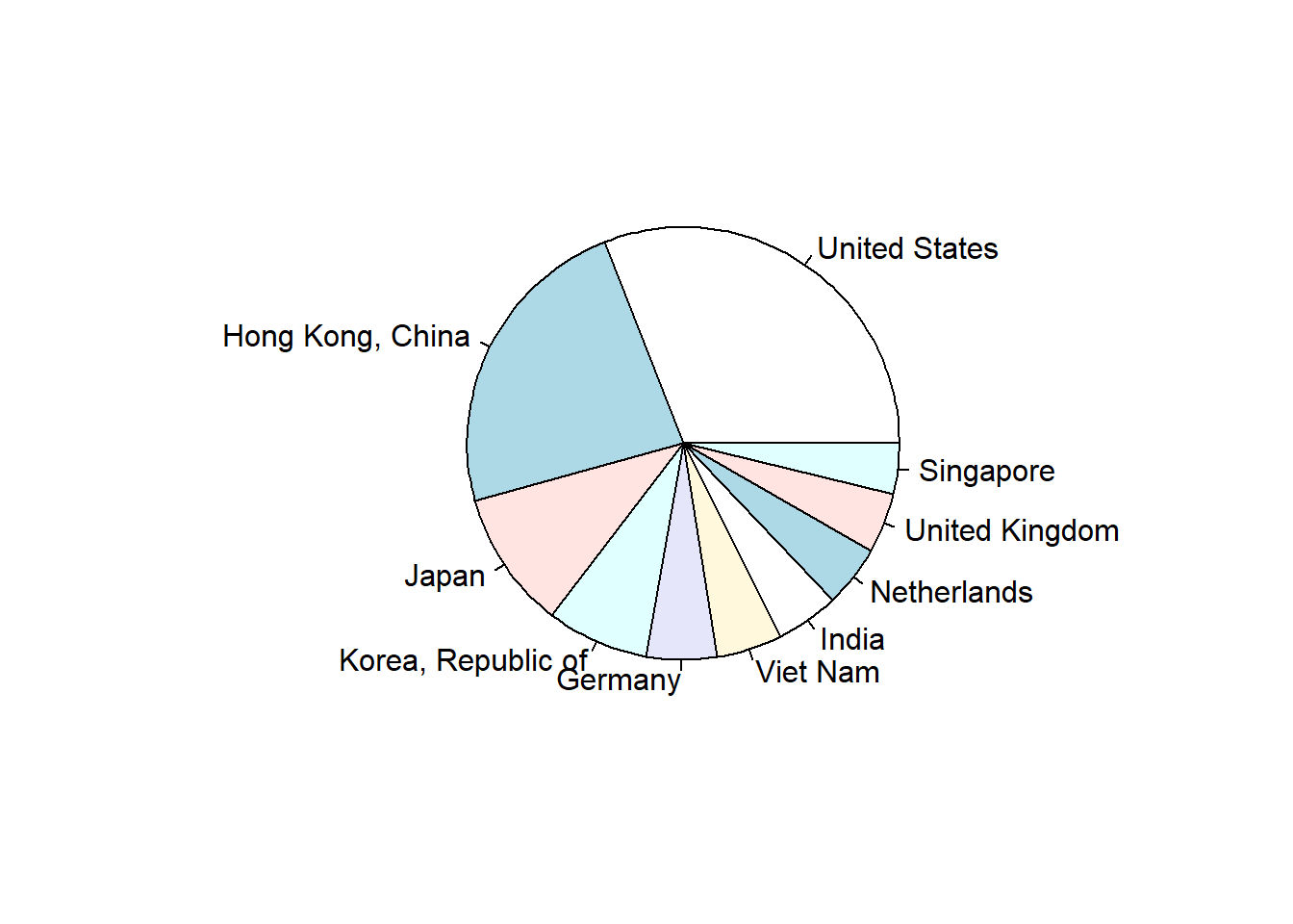
We can also make a bar plot with the barplot command. We specify the color to be the same for the same regions: col=CNX_merged_top10$region.
barplot(CNX_merged_top10$value,
names=CNX_merged_top10$country,
col=CNX_merged_top10$region)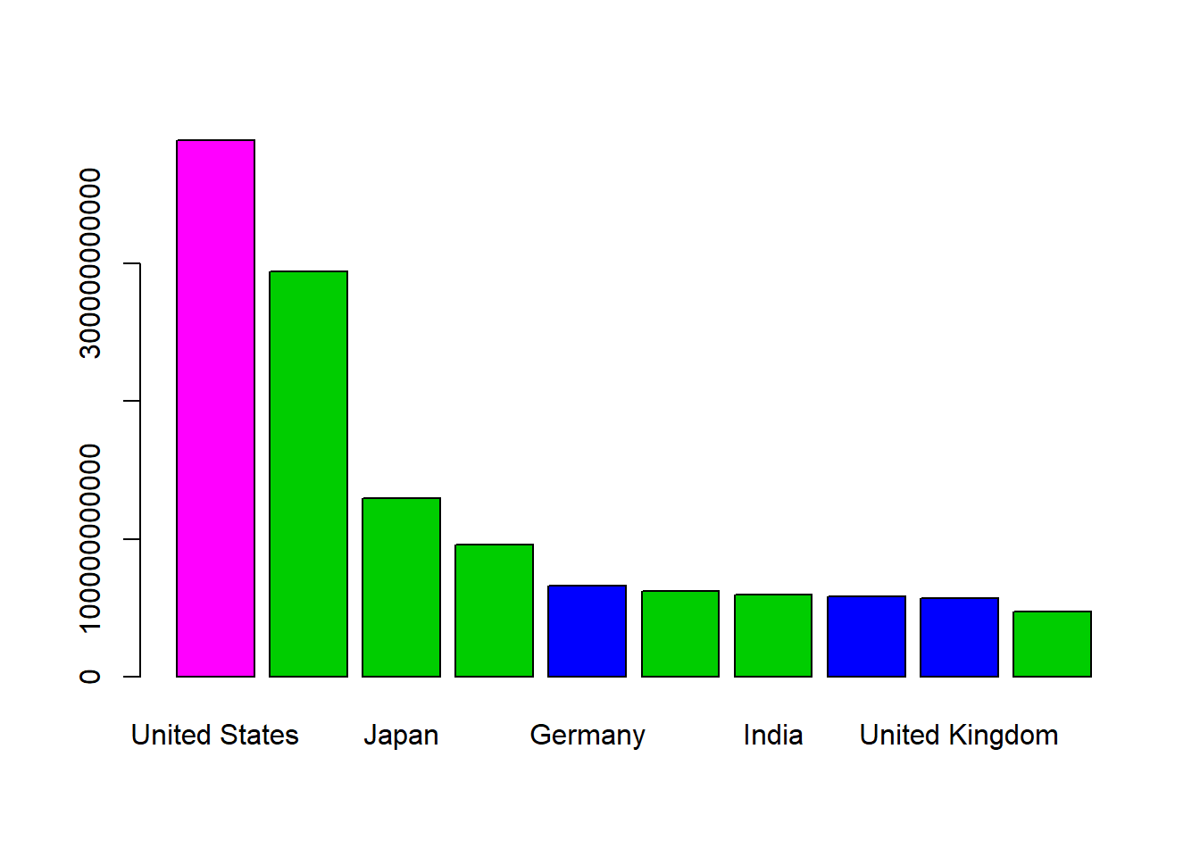
Let’s do one more example before going to the loop subsection. We can do the same graphics for the Philippines (566) for 2016.
We first subset export data for the Philippines for 2016 not to the world.
PH_X_countries <-
trade_data[trade_data$flow=="E"&
trade_data$reporter==566&
trade_data$year==2016&
trade_data$partner!=1,]

head(PH_X_countries)
## reporter flow partner year value
## 1081095 566 E 112 2016 475800328
## 1081100 566 E 158 2016 11674107669
## 1081102 566 E 542 2016 2095041077
## 1081103 566 E 544 2016 684932
## 1081108 566 E 343 2016 429046
## 1081109 566 E 433 2016 14130931We merge the exports to countries with the codes data set:
PHX_merged <- merge(PH_X_countries,
codes, by.x="partner",
by.y="code")
PHX_merged <- PHX_merged[PHX_merged$isCountry==1, c("country", "value", "isCountry","region")]

head(PHX_merged)
## country value isCountry region
## 4 United States 8670654131 1 North America
## 5 United Kingdom 475800328 1 Europe
## 6 Austria 67115695 1 Europe
## 7 Belgium 399641671 1 Europe
## 8 Denmark 35623543 1 Europe
## 9 France 726782604 1 EuropeWe sort the data frame based on value in descending order:
PHX_merged <- PHX_merged[order(-PHX_merged$value),]

head(PHX_merged)
## country value isCountry region
## 18 Japan 11674107669 1 Asia Pacific
## 4 United States 8670654131 1 North America
## 97 Hong Kong, China 6582766881 1 Asia Pacific
## 190 China 6192432905 1 Asia Pacific
## 109 Singapore 3700590527 1 Asia Pacific
## 10 Germany 2293130299 1 EuropeWe select the top 10 export destinations and create a bar plot.
PHX_merged_top10 <- head(PHX_merged,10)

barplot(PHX_merged_top10$value,
names=PHX_merged_top10$country,
col=PHX_merged_top10$region,
main="PHL")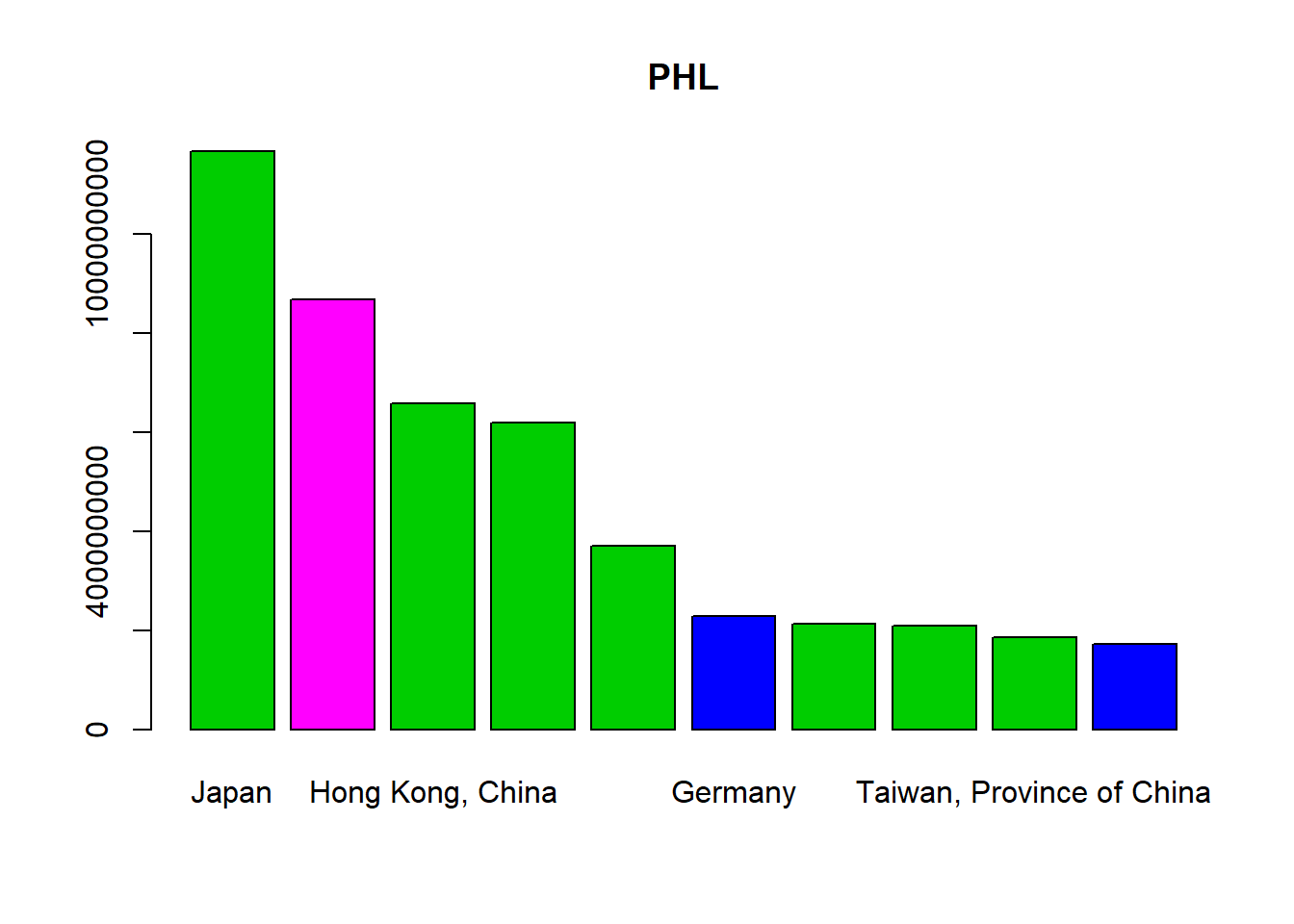
We can select the country name of the Philippines based on its code 566:
codes[codes$code==566,"country"]## [1] Philippines
## 245 Levels: Advanced Economies (IMF) Afghanistan Africa ... ZimbabweSo now we can include the country name in the bar plot:
barplot(PHX_merged_top10$value,
names=PHX_merged_top10$country,
col=PHX_merged_top10$region,
main=codes[codes$code==566,"country"],
las=2) # makes label text perpendicular to axis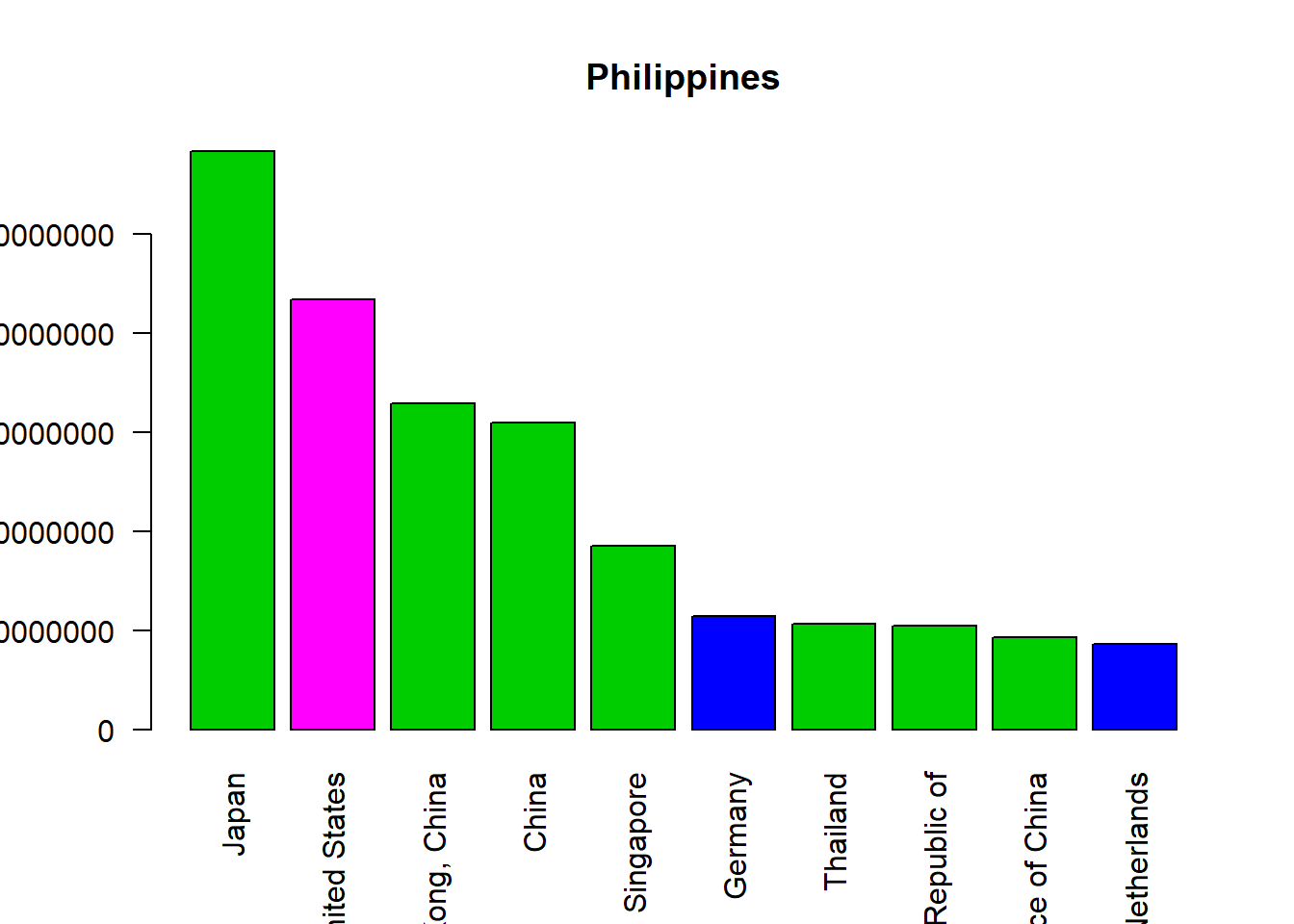
The option las = 2 specifies where the title should be, 2 is for “always perpendicular to the axis”. Once again, more options can be found in ?par.
This does not fit very well, so we specify the par command with mar which controls the margins. You have to play with it until it fits.
par(mar=c(11,8,1,1))
barplot(PHX_merged_top10$value,
names=PHX_merged_top10$country,
col=PHX_merged_top10$region,
main=codes[codes$code==566,"country"],
las=2)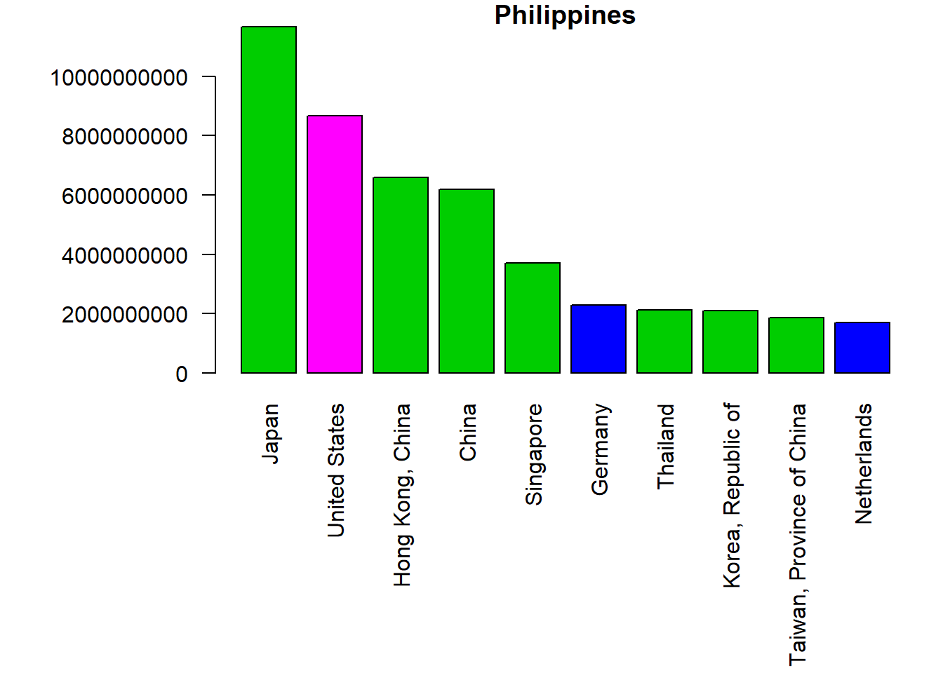
We can save this as a png file with the png command.
png(filename="exports.png") #give the file a name
par(mar=c(11,8,1,1)) #specify margins
barplot(PHX_merged_top10$value,
names=PHX_merged_top10$country,
col=PHX_merged_top10$region,
main=codes[codes$code==566,"country"],
las=2) # makes label text perpendicular to axis

dev.off()
## png
## 2The dev.off() code is very important as without it, your plot will not be saved. (In fact, the plot is not created in your working directory until you run dev.off().)
Quiz
Practice by making a top 10 export destination bar plot of your own country. Add a title, change units, add y axis name and try rotating country names 90 degrees. (Hint: Check the “codes” data set to locate your country and check how we did this for China.)
Your plot should resemble the plot for the Philippines.
#First, check "codes" for your country's code. For the moment we assume your country is ABC and the code is XYZ. If you want to replicate this, make sure you replace ABC with your country's name and XYZ - with the code.
ABC_X_countries <- trade_data[trade_data$flow=="E"&
trade_data$reporter==XYZ&
trade_data$year==2017&
trade_data$partner!=1,]

# we merge the trade data with the codes data set in order to have the trade value matched to the reporter's country name, region and isCountry
ABC_X_merged <- merge(ABC_X_countries,
codes, by.x="partner",
by.y="code")
ABC_X_merged <- ABC_X_merged[ABC_X_merged$isCountry==1, c("country", "value", "isCountry","region")]

# order all data in descending order, remeber NOT to forget the "-" (minus) otherwise you will get the data in ascending order
ABC_X_merged <- ABC_X_merged[order(-ABC_X_merged$value),]

# we get the top 10 countries
ABC_X_merged_top10 <- head(ABC_X_merged,10)

# we construct the bar plot, don't forget to put the name of your country instead of "ABC"
par(mar=c(11,8,1,1))
barplot(ABC_X_merged_top10$value,
names=ABC_X_merged_top10$country,
col=ABC_X_merged_top10$region,
main="ABC", las=2)
3.3 Loop with countries
This is a loop:
for (c in 1:3){
print(c*5)
}
## [1] 5
## [1] 10
## [1] 15We specify that a variable c should be between 1 and 3 inclusive. We then multiply this value with 5, each time this is the done, the loop moves to the next item. This is called an iteration. When c=1, it multiplies c with 5, prints a result (i.e. 5) and then iterates to c=2, and like this until c=3 is multiplied with 5, where we have defined the upper bound.
Study well the syntax and the usage of brackets. Once done, do the quiz below!
Quiz
What is the correct specification if we want to loop through numbers from 2 to 5 and print out those values times 2? (Hint: Study first these code and look at the above code. Hint 2: Run each one to see what happens.)
for (c in 2:5){
print(c)
}
#Answer A is incorrect because we only print the c value, without multiplying it by 2 as required. Therefore answer B is the correct answer. for (c in 2:5){
print(c*2)
}
#Answer B is correct. Good job! for (c in 2:5){
print(c*2)
#Answer C is incorrect because we are missing a bracket at the end! Notice the syntax of a for loop: for (condition) {code to be executed}. Hence, the correct answer is Answer B.for c in 2:5 {
print(c*2)
}
#Answer D is incorrect for a similar reason as C, but here we have failed to put the condition inside brackets. Answer B is the same but in brackets, hence it is the correct answer. 3.4 Loops continued
We can use a loop to create bar plots for all countries all at once! This is great because it saves us time and space! In fact, that is why loops are very popular.
So let’s make a loop that creates bar plots for different countries all at once. We will use the exact same code as the China and Philippines examples. The Philippines example is shown below. Check the comments in the code to remind yourself how we make the bar plot!
# create data subset with Philippine exports to countries in 2016
PH_X_countries <-
trade_data[trade_data$flow=="E"&
trade_data$reporter==566&
trade_data$year==2016&
trade_data$partner!=1,]

# give the barplot a name and save as png
png(filename="exports.png") #give the file a name
par(mar=c(11,8,1,1)) #specify margins
#bar plot specifications
barplot(PH_X_countries$value,
names=PH_X_countries$partner,
main=codes[codes$code==566,"country"],
las=2) # makes label text perpendicular to axis

dev.off()
So in order to automate this to produce several bar plots we need to make sure in each loop iteration we 1) create a new data subset and 2) update the name of the new bar plot.
Let’s inspect these two points separately, we start with the first one. How would a loop which creates each time a different subset of data per country look like? Let’s look at the case below for the Philippines:
PH_X_countries <-
trade_data[trade_data$flow=="E"&
trade_data$reporter==566&
trade_data$year==2016&
trade_data$partner!=1,]
The line of code selecting the country (trade_data$reporter==566) is the one telling R to make a subset for that country, therefore we need to change this line in order to have a new subset of data in each iteration.
Since we want a different country each time, we need a list of all the unique country codes. We take the unique values of the country codes from the codes data set.
unique_ctry_codes <- codes[codes$isCountry==1,"code"]
head(unique_ctry_codes)
## [1] 512 799 914 612 859 614Now let’s learn how to iterate to create different data sets!
Let’s inspect the code below together line by line. We do this for the first five codes - for(i in 1:5) and iterate over i. This way we create five CN_X_countries data sets. Inside the specifications for the data set CN_X_countries, we select exports - trade_data[trade_data$flow=="E". We then iterate on i in trade_data$reporter==unique_ctry_codes[i]. This means that every time the reporter from the trade_data is equal to one of the codes in unique_ctry_codes, we create the CN_X_countries data set. Putting the square brackets for the list variable unique_ctry_codes gives us access to its values. Finally, we select for the year 2016 - trade_data$year==2016 and say that everyone should be included apart from the world - trade_data$partner!=1.
for(i in 1:5){
CN_X_countries <-
trade_data[trade_data$flow=="E"&
trade_data$reporter==unique_ctry_codes[i]& #
trade_data$year==2016&
trade_data$partner!=1,]
}
So now that we know how to iterate to create different data sets, let’s find out how to iterate in order to get different bar plots!
Once again, this is the code for the bar plot.
png(filename="exports.png")
par(mar=c(11,8,1,1))
barplot(PH_X_countries$value,
names=PH_X_countries$partner,
main=codes[codes$code==566,"country"],
las=2)

dev.off()
What do we have to change in order to have a different bar plot for each different data set?
We need to have the file name (filename="exports.png") changed as we want to save the bar plots under different names. We also want the title (main=codes[codes$code==566,"country"]) changed as well. The rest of the parameters depend on the data subset, so they change with the change in data subset. (Hence, we do not need to change them.)
Let’s start with the second one - changing the bar plot title. We can change this the same way we changed trade_data$reporter==566 to trade_data$reporter==unique_ctry_codes[i]. In this case we change main=codes[codes$code==566,"country"] to main=codes[codes$code==unique_ctry_codes[i],"country"].
For the file name, it is a bit more complicated as we not only need to have the name of the country (codes[codes$code==unique_ctry_codes[i],"country"]) but also .png.
We can use paste0 to join the country name with “.png” and convert this to character type. This would change the code from filename="exports.png" to filename=paste0( codes[codes$code==unique_ctry_codes[i],"country"], ".png" ).
We combine the subset code with the new code for the bar plot and test our loop:
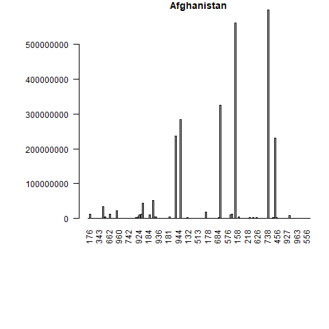
for(i in 1:5){
CN_X_countries <-
trade_data[trade_data$flow=="E"&
trade_data$reporter==unique_ctry_codes[i]&
trade_data$year==2016&
trade_data$partner!=1,]

png(filename=paste0(
codes[codes$code==unique_ctry_codes[i],"country"], ".png"
))
par(mar=c(11,8,1,1))
barplot(CN_X_countries$value,
names=CN_X_countries$partner,
main=codes[codes$code==unique_ctry_codes[i],"country"],
las=2)

dev.off()
}
Error in plot.window(xlim, ylim, log = log, …) :
need finite ‘xlim’ values
In addition: Warning messages:
1: In min(w.l) : no non-missing arguments to min; returning Inf
2: In max(w.r) : no non-missing arguments to max; returning -Inf
3: In min(x) : no non-missing arguments to min; returning Inf
4: In max(x) : no non-missing arguments to max; returning -Inf
This gives an error and most likely means that at least one of our data sets created is empty and therefore the graph cannot be created. Don’t worry! We can fix this. Let’s start by inspecting the different data sets created. How can we check if a data set is empty? We can check the number of rows for each data set with nrow and print this using the print command:
for(i in 1:5){
CN_X_countries <-
trade_data[trade_data$flow=="E"&
trade_data$reporter==unique_ctry_codes[i]&
trade_data$year==2016&
trade_data$partner!=1,]

print(nrow(CN_X_countries))
}
## [1] 135
## [1] 0
## [1] 130
## [1] 137
## [1] 98We see that the second data set has zero rows. When we inspect the code, we notice that this corresponds to “Africa not specified” and therefore not a country and not in our trade_data. When a code not belonging to a country is found, the data set CN_X_countries is still created but is empty (nrow(CN_X_countries) is 0). In order to skip this data set and move to the next one, we can create an if statement to check if the data set is empty: if (nrow(CN_X_countries)==0){...}. If this is true, we iterate to the next value in line - if (nrow(CN_X_countries)==0){next}. In R the next command skips the current iteration of a loop and goes to the next one.
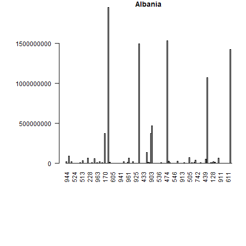
We can update the above loop as such:
for(i in 1:5){
CN_X_countries <-
trade_data[trade_data$flow=="E"&
trade_data$reporter==unique_ctry_codes[i]&
trade_data$year==2016&
trade_data$partner!=1,]

if (nrow(CN_X_countries)==0){next}

print(nrow(CN_X_countries))
}
## [1] 135
## [1] 130
## [1] 137
## [1] 98Now all the data sets have observations, so we can add the if statement to the loop where we subset the data and create bar plots:
for(i in 1:5){
CN_X_countries <-
trade_data[trade_data$flow=="E"&
trade_data$reporter==unique_ctry_codes[i]&
trade_data$year==2016&
trade_data$partner!=1,]

if (nrow(CN_X_countries)==0){next}

png(filename=paste0(
codes[codes$code==unique_ctry_codes[i],"country"], "2.png"
))
par(mar=c(11,8,1,1))
barplot(CN_X_countries$value,
names=CN_X_countries$partner,
main=codes[codes$code==unique_ctry_codes[i],"country"],
las=2)

dev.off()
}
What if we want to have bar plots with the top 10 importers? The logic is the same, however we have two more steps! We have to put the trade value in descending order and merge the data trade values with the names and regions of the partners.
Let’s do this for only the first 5 elements from the unique_ctry_codes data set. We begin by setting the loop and creating a CN_X_countries data set in each loop. We merge this data set with the codes data set to get the country names and regions. We order the merged data and select the top 10 exporter destinations in highest value. Finally we create a bar plot.
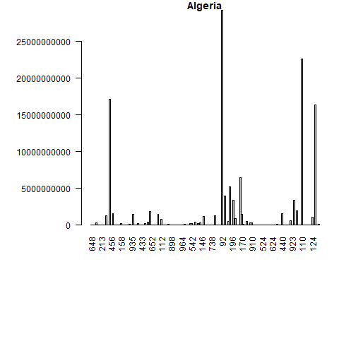
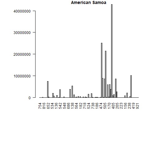
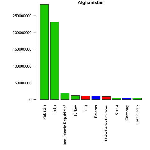
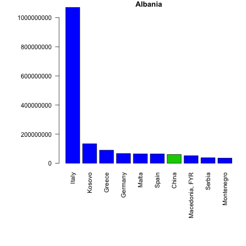
Let’s see the loop first and the created bar plots. Don’t worry, a more detailed explanation follows after.
f <- 5
for(i in 1:f){

CN_X_countries <-
trade_data[trade_data$flow=="E"&
trade_data$reporter==unique_ctry_codes[i]&
trade_data$year==2016&
trade_data$partner!=1,]
if (nrow(CN_X_countries)==0){next}

#we merge reporter countries' exports to the codes data set

CNX_merged <- merge(CN_X_countries,
codes, by.x="partner",
by.y="code")
CNX_merged <- CNX_merged[CNX_merged$isCountry==1, c("country", "value", "isCountry","region")]

#sort the data in descening order

CNX_merged <- CNX_merged[order(-CNX_merged$value),]

#select top 10 export destinations

CNX_merged_top10 <- head(CNX_merged,10)

png(filename=paste0(
codes[codes$code==unique_ctry_codes[i],"country"], ".png"
))
par(mar=c(11,8,1,1))
barplot(CNX_merged_top10$value,
names=CNX_merged_top10$country,
col=CNX_merged_top10$region,
main=codes[codes$code==unique_ctry_codes[i],"country"],
las=2)
dev.off()
}
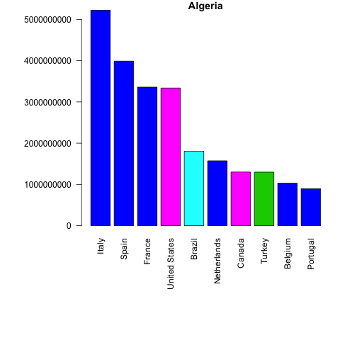
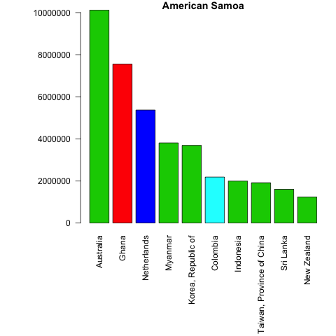
Let’s inspect the code in detail.
Once again our loop goes from 1 until 5 (f <- 5 for(i in 1:f){...}), but we only get 4 barplots. This is because one of our five elements is not a country. To control for empty datasets we use an if statement and move to the next iteration if an empty dataset is found - if (nrow(CN_X_countries)==0){next}.
From then on, we proceed as before. We merge the exports data with the codes data in order to have the corresponding country names: CNX_merged <- merge(CN_X_countries, codes, by.x="partner", by.y="code"). We select the variables we want: CNX_merged <- CNX_merged[CNX_merged$isCountry==1, c("country", "value", "isCountry","region")] , order the data: CNX_merged <- CNX_merged[order(-CNX_merged$value),] and choose the top 10 country export destinations: CNX_merged_top10 <- head(CNX_merged,10).
If you want bar plots for all countries available - equate f <- nrow(unique_ctry_codes). (Giving a variable for our loop upper bound gives us the liberty to change this value easily.)
Good job! In the Section 4 we will learn how to make even better plots!
3.4.1 Quiz
Which lines would you change in the above loop to have 15 elements through which we want to loop and show top 5 export destinations? (Hint: have a good look at the code above! Hint 2: try out the options below and see what you get!)
A. f <- 15
CNX_merged_top5 <- head(CNX_merged,5)
#Answer A is incorrect because we forgot to change the specification of the barplot. Answer C is the same as A, except it adds the correct barplot specifications, hence the correct answer in this case. B. CNX_merged_top5 <- head(CNX_merged,5)
barplot(CNX_merged_top5$value,
names=CNX_merged_top5$country,
col=CNX_merged_top5$region,
main=codes[codes$code==unique_ctry_codes[i],"country"],
las=2)
#Answer B is incorrect because we forgot to change the value for f! Answer C has this, hence it is the correct answer. C. f <- 15 CNX_merged_top5 <- head(CNX_merged,5)
barplot(CNX_merged_top5$value,
names=CNX_merged_top5$country,
col=CNX_merged_top5$region,
main=codes[codes$code==unique_ctry_codes[i],"country"],
las=2)
#Answer C is correct. Good job!