Estimating Ad-valorem Equivalents (AVEs) of Non-tariff Measures (NTMs)
1 Non-tariff Measures (NTMs): overview and data files
If you are not familiar with R, we highly recommend you take this short (free) self-paced online course on using R for analysis of NTMs and trade data here.
Typically, NTMs are more complex, less transparent and, due to their technical nature, are often more difficult to monitor and challenge than tariffs. To learn more about NTMs, we highly recommend this publication.
However, it is sometimes convenient to represent the costs on NTMs in units equivalent to ad-valorem tariffs. Furthermore, one advantage of the price-based AVE estimation method described here is that the AVEs can be immediately used in the GTAP model, without the need to adjust them based on import-demand elasticities, permitting assessment of the impacts of NTM harmonization policies at bilateral, plurilateral or regional level, among other scenarios aiming to study the effects of NTMs.
This online guide is designed to accompany New Price-based Bilateral Ad-valorem Equivalent Estimates of Non-tariff Measures to allow researchers to replicate the results as well as re-estimate AVEs under different assumptions or methods. 95% of work has been putting the data together. You’re welcome.
In the table below you can find the datasets we will use.
| Description | File name | Link to download |
|---|---|---|
| HS6-GTAP concordance (commodity) [~71 KB] | HS12-gtap.csv | here |
| GTAP-ISO3 concordance (country) [~5 KB] | gtap_iso_concordance.csv | here |
| Detailed trade and NTMs data [~283,480 KB] | merged-11-April-2020.zip | here |
1.1 Data cleaning and regression
Import the packages we are going to need to use and set some global parameters.
#import packages
library("car")
library("stringi")
library("stringr")
library("dplyr")
library("data.table")
library("sandwich")
library("lmtest")
#set global parameters
options(warn=1)
options(scipen = 999) #removes scientific notation
Next, load the concordance file with HS six-digit codes and their corresponding GTAP sectors, HS chapters (two digits) and sections.
com_con <- read.csv("HS12-gtap.csv", stringsAsFactors = FALSE)
#note stringsAsFactors is FALSE by default in the latest R version but you may still need it if you use an older version
Unzip the “merged-11-April-2020.zip” files and put them into one directory (avoid putting other files there). Import all the HS six-digit csv data file names from the unzipped folder and store them in a new dataframe variable, hs_detailed. This will help us access corresponding files in loops described later. dir() can list all the file names in a given directory which will be specified by its argument, path. pattern is an optional argument that records file names which match the regular expression it receives. stringr::str_split_fixed(files, "[.]", 2)[,1] slices all the file names into two parts and only retains the first part (six digits).
files <- dir(path = "C:/Users/Alexi/OneDrive - United Nations/_R/aves/merged-11-April-2020", pattern = "\\.csv$")

#the path should specify where all the unzipped csv files are, e.g. '010121.csv','010129.csv',..
#if you get an error or an empy frame, your folder path is probably wrong

hs_detailed <- data.frame(hs6 = stringr::str_split_fixed(files, "[.]", 2)[,1])

nrow(hs_detailed) #number of CSV files you should have in the unzipped folder
## [1] 5203head(hs_detailed)## hs6
## 1 010121
## 2 010129
## 3 010130
## 4 010190
## 5 010221
## 6 010229Next, we add a leading zero to the HS six-digit codes incom_con to make them all 6 digits (to match the leading zeros in the unzipped file names, otherwise codes without leading zeros e.g. chapter 9 and below get truncated). We then merge hs_detailed with com_con by hs6. The result would be that each existing csv file (corresponding to individual HS six-digit code) will have a concordance to chapter, section and GTAP sector for later use.
com_con$hs6 <-  stri_pad_left(com_con$hs6,6,0)
hs_detailed <- merge(hs_detailed, com_con, by="hs6", all.x = TRUE)
head(hs_detailed)
## hs6 section chapter gtap
## 1 010121 1 1 ctl
## 2 010129 1 1 ctl
## 3 010130 1 1 ctl
## 4 010190 1 1 ctl
## 5 010221 1 1 ctl
## 6 010229 1 1 ctlWe create two lists to store detailed interaction coefficients of technical measures and non-technical measures. We also create a new vector, chapters, that stores all the unique values of chapter column (HS two-digit chapters) of hs_detailed. chapters will be used to create a for loop in the following steps, i.e. the number of regressions run will be equal to the number of unique HS chapters (HS two-digit codes). Note you can instead estimate by section - just change the corresponding instances from chapter to section (or even GTAP sector straight away - but the GTAP sector sizes are less balanced in product groupings).
hs_beta_list <- vector("list", nrow(hs_detailed))
names(hs_beta_list) <- hs_detailed$hs6

hs_beta_list_nt <- vector("list", nrow(hs_detailed))
names(hs_beta_list_nt) <- hs_detailed$hs6

chapters <- unique(hs_detailed$chapter)

# defining EU countries (2015 so pre-Brexit)
EUN <- c('AUT', 'BEL', 'BGR', 'HRV', 'CYP', 'CZE', 'DNK', 'EST', 'FIN', 'FRA', 'DEU', 'GRC', 'HUN', 'IRL', 'ITA', 'LVA', 'LTU', 'LUX', 'MLT', 'NLD', 'POL', 'PRT', 'ROM', 'SVK', 'SVN', 'ESP', 'SWE', 'GBR')
Before creating the for loop, a dataframe is created to store the summary statistics of the regressions. We also define two parameters here, which you are able to change according to your preferences/assumptions. n denotes the percentage of derived prices (value/quantity) you want to truncate (top or/and bottom). both denotes whether you want to remove the bottom n% of derived prices as well as top. Three are, unfortunately some real outliers that significantly affect the results if this step is skipped.
results_summary <- data.frame(matrix(vector(),0,12,
                              dimnames = list(c(),
                              c("chapter",
                                "ntm_count_t_b",
                                "ntm_count_nt_b",
                                "ntm_count_t_p",
                                "ntm_count_nt_p",
                                "ntm_count_t_int",
                                "ntm_count_t_int_sign",
                                "ntm_count_nt_int",
                                "ntm_count_nt_int_sign",
                                "n",
                                "r",
                                "adj")
                              )),
                              stringsAsFactors=F)

n <- 5; both = FALSE
#feel free to experiment with these; do sensitivity analysis
Next, let’s load all the HS six digit data files in the folder and run regressions on them with a loop. Please note that this chunk may take more than an hour or so to run (depending on your system). If you have a particularly powerful machine with A LOT of RAM, you can try to merge all CSVs and run it as one regression. Let me know if you succeed I will be most interested. In this application they are run at chapter level (96 regressions).
for(s in 1:length(chapters)){
  merged5 <- data.frame()

  subsetx <- hs_detailed[hs_detailed$chapter==chapters[s],]
  for(f in 1:nrow(subsetx))
  {
    hs_code <- subsetx[f,"hs6"]
    cat( "--- hs code: ",hs_code," ---\n");flush.console()
    merged4 <- read.csv(paste0(hs_code,".csv"), stringsAsFactors = FALSE)

    #remove Inf or NA prices
    merged4 <- merged4[!is.na(merged4$price)&merged4$price<Inf,]

    #truncate top (and bottom) n of prices (5%)
    merged4 <- merged4[merged4$price<quantile(merged4$price,prob=1-n/100),]
    if(both==TRUE){
      #note if you you to truncate both min and max prices outliers, change the "both" parameter above to TRUE
      merged4 <- merged4[merged4$price>quantile(merged4$price,prob=n/100),]
    }

    #token - unit, https://comtrade.un.org/data/MethodologyGuideforComtradePlus.pdf, table 3
    if(length(unique(merged4$QtyToken))>1){
      sum_q <- merged4 %>% group_by(QtyToken)%>% count()

      #only choose the rows with the most frequent quantity token
      merged4 <- merged4[merged4$QtyToken==as.numeric(sum_q[which.max(sum_q$n),"QtyToken"]),]
      if(length(unique(merged4$QtyToken))>1){
        stop("Too many q tokens again")
      }
    }
    if(nrow(merged4)>0){
      if(nrow(merged5)==0){
        merged5 <- merged4
        #lazy way to create a new dataframe for rowbinding, sorry
      }else{
        nextrow = nrow(merged5)+1
        merged5[nextrow:(nextrow+nrow(merged4)-1),] = merged4
        # we need to assure unique row names
        row.names(merged5) = 1:nrow(merged5)
      }
    }
  }

  cat( "---CHAPTER: ",s," : RUNNING REGRESSION---\n");flush.console()

  #Feel free to adjust here to estimate individual ICNTM chapters - this example is based on
  #just groups of technical and non-technical measures

  merged5$ntm_count_t <- merged5$A + merged5$B + merged5$C
  merged5$ntm_count_nt <- merged5$E + merged5$F + merged5$G + merged5$H + merged5$I

  # removing intra-EU NTMs
  merged5[(merged5$ReporterISO3 %in% EUN)&(merged5$PartnerISO3 %in% EUN),c("ntm_count_t", "ntm_count_nt")] <- 0


  reg1 <- lm(log(price) ~
               log(dist) + contig + comlang_off + rta + llocked +
               applied + ntm_count_t +
               ntm_count_nt +
               factor(ProductCode)+
               ReporterISO3 +
               PartnerISO3
             + ReporterISO3*ntm_count_t
             + ReporterISO3*ntm_count_nt
             ,
             data = merged5)

  #this is individual regression summary, not to be confused with results_summary defined above
  summary_results <-  data.frame(summary(reg1)$coefficients[,c("Estimate","Pr(>|t|)")])

  #vcovCL: Clustered Covariance Matrix Estimation. To get robust errors.
  #Please refer to https://rdrr.io/rforge/sandwich/man/vcovCL.html if you are interested.
  clustered_errors <- coeftest(reg1, vcov = vcovCL, cluster = ~ dist)
  clustered_errors <- data.frame(clustered_errors[1:nrow(summary_results),c(2,4)])
  clustered_errors$coef <- rownames(clustered_errors)

  summary_results$coef <- rownames(summary_results)
  summary_results <- merge(summary_results, clustered_errors, by="coef")
  rownames(summary_results) <- summary_results$coef
  summary_results <- summary_results %>% select(Estimate,`Pr...t...y` ) %>% rename(`Pr...t..` = `Pr...t...y`)
  summary_results <- summary_results[rownames(data.frame(summary(reg1)$coefficients)),]
  rm(clustered_errors)

  #row.names() is more efficient than rownames()
  rownames_1 <- row.names(summary(reg1)$coefficients)

  #regular expression to find anything with ":" - those are interactions
  rownames_1 <- which(rownames_1  %in%  rownames_1[grepl("[:]", rownames_1)]  )
  summary_results <- summary_results[rownames_1,]
  rownames_1 <- row.names(summary_results)
  rownames_1 <- which(rownames_1  %in%  rownames_1[grepl("ntm_count_t", rownames_1)]  )

  summary_results_t <- data.frame(summary_results[rownames_1, ])

  rownames_1 <- row.names(summary_results)
  rownames_1 <- which(rownames_1  %in%  rownames_1[grepl("ntm_count_nt", rownames_1)]  )

  summary_results_nt <- data.frame(summary_results[rownames_1, ])

  # format the list to store and then merge later on
  summary_results_t_for_list <- summary_results_t
  summary_results_t_for_list <- summary_results_t_for_list[!is.na(summary_results_t_for_list$Estimate),]
  summary_results_t_for_list$reporter <- rownames(summary_results_t_for_list)
  summary_results_t_for_list$reporter <- str_sub(summary_results_t_for_list$reporter,-3,-1)
  rownames(summary_results_t_for_list) <- 1:nrow(summary_results_t_for_list)
  summary_results_t_for_list <- summary_results_t_for_list %>% select(reporter, Estimate, `Pr...t..`) %>% rename(p=`Pr...t..`, beta_interaction = Estimate)

  summary_results_nt_for_list <- summary_results_nt
  summary_results_nt_for_list <- summary_results_nt_for_list[!is.na(summary_results_nt_for_list$Estimate),]
  summary_results_nt_for_list$reporter <- rownames(summary_results_nt_for_list)
  summary_results_nt_for_list$reporter <- str_sub(summary_results_nt_for_list$reporter,-3,-1)
  rownames(summary_results_nt_for_list) <- 1:nrow(summary_results_nt_for_list)
  summary_results_nt_for_list <- summary_results_nt_for_list %>% select(reporter, Estimate, `Pr...t..`) %>% rename(p=`Pr...t..`, beta_interaction = Estimate)

  # store all the regression results in lists
  for(j in 1:nrow(subsetx))
  {
    hs_codej <- subsetx[j,"hs6"]
    hs_beta_list[[hs_codej]] <- summary_results_t_for_list
    hs_beta_list_nt[[hs_codej]] <- summary_results_nt_for_list

  }
  rm(summary_results_t_for_list, j)

  results_summary[s,"chapter" ] <- chapters[s]
  results_summary[s,"ntm_count_t_b" ] <- summary(reg1)$coefficients[c("ntm_count_t"),"Estimate"]
  results_summary[s,"ntm_count_t_p" ] <- summary(reg1)$coefficients[c("ntm_count_t"),"Pr(>|t|)"]

  summary_results <-  data.frame(summary(reg1)$coefficients[,c("Estimate","Pr(>|t|)")])
  rownames_1 <- row.names(summary_results)
  rownames_1 <- which(rownames_1  %in%  "ntm_count_nt")

  if (length(rownames_1)>0){
    results_summary[s,"ntm_count_nt_b" ] <- summary(reg1)$coefficients[c("ntm_count_nt"),"Estimate"]
    results_summary[s,"ntm_count_nt_p" ] <- summary(reg1)$coefficients[c("ntm_count_nt"),"Pr(>|t|)"]
  }

  results_summary[s,"ntm_count_t_int" ] <- nrow(summary_results_t)
  results_summary[s,"ntm_count_t_int_sign" ] <- nrow(summary_results_t[summary_results_t[,2]<0.1&!is.na(summary_results_t[,2]),])
  results_summary[s,"ntm_count_nt_int" ] <- nrow(summary_results_nt)
  results_summary[s,"ntm_count_nt_int_sign" ] <- nrow(summary_results_nt[summary_results_nt[,2]<0.1&!is.na(summary_results_nt[,2]),])

  results_summary[s,"n" ]   <- nrow(merged5)
  results_summary[s,"r" ]   <- summary(reg1)$r.squared
  results_summary[s,"adj" ] <- summary(reg1)$adj.r.squared
  gc() # garbage collector - frees working memory
}
In the outer for loop, we create an empty dataframe, merged5. Then, one chapter at a time, we create another for loop to load and rowbind all files with HS six digit codes in that chapter in the folder with HS six digit csv files with all the data on NTMs, trade flows, etc, truncate top and bottom n% of prices, keep the most frequent quantity token (unit), and store results in merged5. We calculate the total number of technical measures and non-technical measures respectively and run the following regression:
The following table describes the variables refer to the paper for more details.
| Variable Name | Description | Variable Name (Code) |
|---|---|---|
| \(\delta\) | Fixed effects of country \(i\) and \(j\) | ReporterISO3, PartnerISO3 |
| \(\rho\) | HS6 product fixed effects | factor(ProductCode) |
| \(\theta\) | Pair characteristics (i.e. distance, contiguity, landlocked status, common language, and RTA) | log(dist), contig, llocked, comlang_off, rta |
| \(NTM^{Technical}_{ijk}\) | The count of separate non-tariff measures from chapters A to C imposed by \(i\) on imports of product \(k\) from \(j\) | ntm_count_t |
| \(NTM^{Nontechnical}_{ijk}\) | The count of separate non-tariff measures from chapters D to O imposed by \(i\) on imports of product \(k\) from \(j\) | ntm_count_nt |
| \(tariff_{ijk}\) | Applied tariff (MFN or lowest preferential, if available) imposed by \(i\) on imports of product \(k\) from \(j\) | applied |
We cluster errors based on dist and store them in summary_results. Then, we extract the coefficients of interaction items, divide the results into technical measures summary, summary_results_t, and non-technical measures summary, summary_results_nt, rename row names to country ISO3 codes, and rename columns Pr...t.. and Estimate to p and beta_interaction respectively. Next, we store all the regression results in hs_beta_list and hs_beta_list_nt. In the end of each loop, we save all the information into the summary statistics dataframe we created before, results_summary.
After the loop finishes running (hours), we save results_summary to a csv file.
write.csv(results_summary,"./results_summary.csv", row.names=FALSE)The results_summary data frame should correspond to output in Table A.4 of the journal article Annex.
1.2 Estimating AVEs using coefficients from the regressions
Let’s now proceed to estimating AVEs using the regression coefficients derived in the previous step. To begin with, we create an empty dataframe to store the results:
aves_file_final <- data.table(data.frame(matrix(vector(),0,8,
                                                dimnames =
                                                  list(c(),
                                                       c("ReporterISO3", "PartnerISO3",
                                                         "aves_t","aves_nt", "TradeValue",
                                                         "ntm_count_t", "ntm_count_nt", "hs_code" ))),
                                         stringsAsFactors=F))
We then create a for loop to calculate AVEs. Here, we will follow the following equations (see paper for full details):
\(AVE_{ijk}^{Technical}[total]=\tanh((\exp(\beta_4\times NTM^{Technical}_{ijk}+\beta_{6i} \times NTM^{Technical}_{ijk} )-1))\times100\)
\(AVE_{ijk}^{Nontechnical}[total]=\tanh((\exp(\beta_5 \times NTM^{Nontechnical}_{ijk}+\beta_{7i} \times NTM^{Nontechnical}_{ijk} )-1))\times100\)
Note that we restrict the highest AVEs to 100 through a hyperbolic function as exponential transformation can result in very large numbers - researchers can relax this assumption and set their own limits.
First, we read all the HS six digit files again and summarize all the technical measures and non-technical measures. We select columns ReporterISO3, PartnerISO3, TradeValue, ntm_count_t, and ntm_count_nt. Next, we load \(\beta_4\) and \(\beta_5\), ntm_count_t_b and ntm_count_nt_b, and their \(p\) values, ntm_count_t_p and ntm_count_nt_p, from results_summary. Before we calculate AVE estimates, we should review our datasets and set \(\beta\) values to 0 if their \(p\) values are over 0.1 (again researchers may wish to adjust these). Now we have all the variables in the equation. We calculate AVE estimates for technical and non-technical measures. The results are saved in aves_file_final dataframe we created earlier.
for(f in 1:length(files))
{
  hs_code <- strsplit(files[f]  , "[.]")[[1]][1]
  cat( "--- hs code: ",hs_code," ---\n");flush.console()

  merged4 <- read.csv(files[f], stringsAsFactors = FALSE)

  if (nrow(merged4)==0){next()}
  merged4$ntm_count_t <- merged4$A + merged4$B + merged4$C
  merged4$ntm_count_nt <-  merged4$E + merged4$F + merged4$G + merged4$H + merged4$I

  merged4 <- merged4 %>% select(ReporterISO3, PartnerISO3,TradeValue, ntm_count_t, ntm_count_nt)

  #remove intra-EU tariffs
  merged4[(merged4$ReporterISO3 %in% EUN)&(merged4$PartnerISO3 %in% EUN),c("ntm_count_t", "ntm_count_nt")] <- 0

  chapter <- as.numeric(substr(hs_code, start = 1, stop = 2))

  ntm_count_t_b <- results_summary[results_summary$chapter==chapter,c("ntm_count_t_b")]
  ntm_count_t_p <- results_summary[results_summary$chapter==chapter,c("ntm_count_t_p")]

  ntm_count_nt_b <- results_summary[results_summary$chapter==chapter,c("ntm_count_nt_b")]
  ntm_count_nt_p <- results_summary[results_summary$chapter==chapter,c("ntm_count_nt_p")]

  if(length(ntm_count_nt_p)==0){next()}
  #Why don't we test the length of ntm_count_t_p?
  #If a country does not have technical measures, it will not have non-technical measures and will not be recorded here,
  if(ntm_count_t_p>0.1){ntm_count_t_b <- 0}
  if(ntm_count_nt_p>0.1){ntm_count_nt_b <- 0}

  rm(ntm_count_t_p, ntm_count_nt_p)

  merged4 <- merge(merged4, hs_beta_list[[hs_code]], by.x="ReporterISO3", by.y="reporter", all.x = TRUE)
  if (nrow(merged4)==0){next()}
  merged4[!is.na(merged4$p)&merged4$p>0.1, "beta_interaction"] <- 0
  merged4 <- merged4 %>% rename(beta_interaction_t = beta_interaction) %>% select(-c(p))

  merged4 <- merge(merged4, hs_beta_list_nt[[hs_code]], by.x="ReporterISO3", by.y="reporter", all.x = TRUE)

  if (nrow(merged4)==0){next()}
  merged4[!is.na(merged4$p)&merged4$p>0.1, "beta_interaction"] <- 0
  merged4 <- merged4 %>% rename(beta_interaction_nt = beta_interaction) %>% select(-c(p))

  merged4$aves_t <- tanh(exp(ntm_count_t_b*merged4$ntm_count_t + merged4$beta_interaction_t*merged4$ntm_count_t) - 1)*100
  merged4$aves_t[merged4$aves_t<0] <- 0

  merged4$aves_nt <- tanh(exp(ntm_count_nt_b*merged4$ntm_count_nt + merged4$beta_interaction_nt*merged4$ntm_count_nt) - 1)*100
  merged4$aves_nt[merged4$aves_nt<0] <- 0

  merged4 <- merged4 %>% select(ReporterISO3, PartnerISO3, aves_t, aves_nt, TradeValue, ntm_count_t, ntm_count_nt)

  merged4$hs_code <- hs_code

  l = list(aves_file_final,merged4)
  aves_file_final <- rbindlist(l)
}
To get the global averages, run:
aves_file_final %>%
summarise(ave_t_weighted = weighted.mean(aves_t, TradeValue, na.rm = TRUE),
ave_nt_weighted = weighted.mean(aves_nt, TradeValue, na.rm = TRUE)
)
## ave_t_weighted ave_nt_weighted
## 1 7.179849 6.062699You can visualize the distributions using ggplot function:
#to reshape the data file into a long format for use in ggplot next:
library("reshape2")
long <- melt(aves_file_final[,c("ReporterISO3", "PartnerISO3", "hs_code","aves_t", "aves_nt")], id.vars=c("ReporterISO3", "PartnerISO3", "hs_code"))


library("ggplot2")
ggplot(long, aes(x=value, color=variable )) +
  geom_histogram(alpha=0.5, position="identity")+scale_y_log10()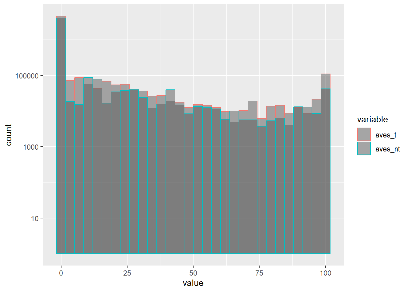
Note I used log transformation for y-axis here as the vast majority of AVEs are quite close to zero.
1.3 AVE estimates for GTAP sectors and regions
Now let’s adjust the AVE database we calculated to make it usable in the GTAP database. We should already have the hs six-digit to sector concordance loaded (hs_detailed). First we merge the ave dataset with gtap sector codes.
#making sure both are numeric, otherwise trailing zeros sometimes cause issues
aves_file_final$hs_code <- as.numeric(aves_file_final$hs_code)
hs_detailed$hs6     <- as.numeric(hs_detailed$hs6)

gtap_aves <- merge(aves_file_final, hs_detailed[,c("hs6","gtap")], by.x="hs_code", by.y="hs6") %>% rename(sector=gtap)
head(gtap_aves)
## hs_code ReporterISO3 PartnerISO3 aves_t aves_nt TradeValue ntm_count_t
## 1: 10121 ARE AUS NA NA 133.609220 7
## 2: 10121 ARE URY NA NA 741.354996 7
## 3: 10121 ARE BEL NA NA 8.509452 7
## 4: 10121 ARE DEU NA NA 1434.923757 7
## 5: 10121 ARE ESP NA NA 22.443169 7
## 6: 10121 ARE ZAF NA NA 250.453571 8
## ntm_count_nt sector
## 1: 3 ctl
## 2: 3 ctl
## 3: 3 ctl
## 4: 3 ctl
## 5: 3 ctl
## 6: 3 ctlNext we load the GTAP region to ISO3 concordance, and merge it for both partners and reporters (and rename them accordingly).
reg_con <- read.csv("gtap_iso_concordance.csv", stringsAsFactors = FALSE)
head(reg_con)
## iso3 gtap_r country
## 1 AFG xsa Afghanistan
## 2 ALB alb Albania
## 3 DZA xnf Algeria
## 4 ASM xoc American Samoa
## 5 AND xer Andorra
## 6 AGO xac Angola#note you may see some double entries for countries with legacy ISO3 codes, like Romania (ROU & ROM) but this does not affect the subsequent aggregations - only affects partner trade in some cases.
gtap_aves <- merge(gtap_aves, reg_con[,c("iso3","gtap_r")], by.x="ReporterISO3", by.y="iso3", all.x = TRUE) %>% rename(reporter = gtap_r)
gtap_aves <- merge(gtap_aves, reg_con[,c("iso3","gtap_r")], by.x="PartnerISO3", by.y="iso3", all.x = TRUE) %>% rename(partner = gtap_r)
head(gtap_aves)## PartnerISO3 ReporterISO3 hs_code aves_t aves_nt TradeValue ntm_count_t
## 1: ABW ARE 392329 NA NA 0.0272294 0
## 2: ABW ATG 950699 NA NA 1.1850000 0
## 3: ABW AUT 852349 7.471075 0.00000 0.8062939 5
## 4: ABW AUT 901839 0.000000 23.97609 1.8876370 12
## 5: ABW BEL 271019 0.000000 0.00000 0.0940000 3
## 6: ABW BEL 681599 0.000000 0.00000 0.0030000 2
## ntm_count_nt sector reporter partner
## 1: 0 crp are xcb
## 2: 0 omf xcb xcb
## 3: 1 crp aut xcb
## 4: 2 ome aut xcb
## 5: 4 p_c bel xcb
## 6: 0 nmm bel xcbWe finally summarize/group trade-weighted means of all indicators by GTAP sectors and regions:
aves_file_final_gtap <- gtap_aves %>% group_by(reporter, partner, sector) %>%
  summarise(ave_t_weighted = weighted.mean(aves_t, TradeValue, na.rm = TRUE),
            ave_nt_weighted = weighted.mean(aves_nt, TradeValue, na.rm = TRUE),
t_count_weighted = weighted.mean( ntm_count_t, TradeValue, na.rm = TRUE),
nt_count_weighted = weighted.mean(ntm_count_nt, TradeValue, na.rm = TRUE),
            TradeValue=sum(TradeValue, na.rm = TRUE)
            )
aves_file_final_gtap
## # A tibble: 218,788 × 8
## # Groups: reporter, partner [12,769]
## reporter partner sector ave_t_weighted ave_nt_weigh…¹ t_cou…² nt_co…³ Trade…⁴
## <chr> <chr> <chr> <dbl> <dbl> <dbl> <dbl> <dbl>
## 1 are alb crp NaN NaN 2.18 1.01 4.04e+0
## 2 are alb fmp NaN NaN 0 0 1.46e+2
## 3 are alb i_s NaN NaN 0 0 1.04e+3
## 4 are alb lea NaN NaN 4.73 0 9.57e+2
## 5 are alb lum NaN NaN 0.0277 0.0830 2.30e+1
## 6 are alb mvh NaN NaN 1 3 2.20e+0
## 7 are alb nmm NaN NaN 0 0 6.59e-1
## 8 are alb ocr NaN NaN 28 6 1.59e+1
## 9 are alb ome NaN NaN 0.954 2.86 1.20e+1
## 10 are alb omf NaN NaN 1.89 0.130 3.15e+1
## # … with 218,778 more rows, and abbreviated variable names ¹ave_nt_weighted,
## # ²t_count_weighted, ³nt_count_weighted, ⁴TradeValue1.4 Filling the gaps
As discussed in the paper, for various reasons there are data gaps (lack of NTM data for countriess, small sample in bilateral trade flows, multicollinearity, etc). Researchers may still wish to fill in these gaps for use in GTAP. This is one such proposed ways. You’d need full matrix of GTAP regions and sectors and create a full data matrix to start with.
| Description | File name | Link to download |
|---|---|---|
| GTAP sector/region level bilateral trade from UN COMTRADE (2015 data) [~6,247 KB] | Totalbilater_gtap_2020.csv | here |
| All GTAP commodities [~1 KB] | set_all_commodities.csv | here |
| All GTAP regions [~2KB] | set_all_regions.csv | here |
Note that in sector/region file there is the most basic concordance between ISO3 codes/HS codes and corresponding GTAP sectors. You may wish to edit these yourselves already if you have a particular aggregation in mind (or follow the steps described in the online annex of the paper)
Totalbilater_gtap <- read.csv("Totalbilater_gtap_2020.csv", stringsAsFactors = FALSE)
#This file contains total bilater trade at gtap sector/region level for 2015
#The column "TotalTrade" is different from the original "TradeValue" as "TradeValue" only includes trade values used in regressions and as noted some were omitted for various reasons

#option to change custom aggregation within these files directly
set_com <- read.csv("set_all_commodities.csv", stringsAsFactors = FALSE)
set_reg <- read.csv("set_all_regions.csv", stringsAsFactors = FALSE)

aves_file_final_gtap <- merge(aves_file_final_gtap, Totalbilater_gtap, by=c("reporter" ,"partner", "sector"), all.x = TRUE)

full_matrix <- data.frame(unique(set_reg$new))
names(full_matrix) <- "reporter_new"
full_matrix <- merge(full_matrix,data.frame(unique(set_reg$new)), all=TRUE)
names(full_matrix)[2] <- "partner_new"
full_matrix <- merge(full_matrix,data.frame(unique(set_com$new)), all=TRUE)
names(full_matrix)[3] <- "sector_new"

full_matrix$index <- 1:nrow(full_matrix)
nrow(full_matrix)
#1117200

length(unique(set_reg$new))*length(unique(set_com$new))*length(unique(set_reg$new))
#1117200 - full GTAP sector x region x region (now empty) matrix

#now merging with iso3 concordances

aves_file_final_gtap <- merge(aves_file_final_gtap, set_reg, by.x = "reporter", by.y = "old", all.x = TRUE)
aves_file_final_gtap <- aves_file_final_gtap %>% dplyr::rename(reporter_new = new)

aves_file_final_gtap <- merge(aves_file_final_gtap, set_reg, by.x = "partner", by.y = "old", all.x = TRUE)
aves_file_final_gtap <- aves_file_final_gtap %>% dplyr::rename(partner_new = new)

aves_file_final_gtap <- merge(aves_file_final_gtap, set_com, by.x = "sector", by.y = "old", all.x = TRUE)
aves_file_final_gtap <- aves_file_final_gtap %>% dplyr::rename(sector_new = new)

full_matrix <- merge(full_matrix, aves_file_final_gtap,
                     by=c("reporter_new", "partner_new", "sector_new"), all.x = TRUE)

#again you could wish to edit edit sector/region files straight away (set_reg, set_com) earlier to get own region/sector aggregation for GTAP - hence "partner, reporter, sector _new" (or use the ready file in the online annex), this will just give you a full matrix (with lots of missing values - not all GTAP sectors/regions have NTM data, regressions don't run to sample sizes, etc)

aves_file_final_gtap <- full_matrix %>% dplyr::group_by(reporter_new, partner_new, sector_new) %>%
  dplyr::summarise(ave_t_weighted = weighted.mean(ave_t_weighted, TradeValue, na.rm = TRUE),
                   ave_nt_weighted = weighted.mean(ave_nt_weighted, TradeValue, na.rm = TRUE),
                   t_count_weighted = weighted.mean(t_count_weighted, TradeValue, na.rm = TRUE),
                   nt_count_weighted = weighted.mean(nt_count_weighted, TradeValue, na.rm = TRUE),
                   TradeValue=sum(TradeValue, na.rm = TRUE),
                   TotalTrade=sum(TotalTrade, na.rm = TRUE))

nrow(aves_file_final_gtap)
#1117200
# if you changed set_reg; set_com files you'd have a different full matrix dimension

aves_file_final_gtap$share <- aves_file_final_gtap$TradeValue/aves_file_final_gtap$TotalTrade*100
#as described in the paper you may wish to remove some NTMs where in some sectors they only cover a small part of total trade share, I personally set it at 30%, but feel free to make your own assumptions (e.g. GTAP services sectors may have one or two HS codes linked to them in concordance, large overall TotalTrade flows, but few would have been have been used in NTM AVE aggregation for the whole GTAP sector)

gtap_imports_final <- aves_file_final_gtap
#personally I like backup datasets along the way in case I mess up and need to re-run the whole thing, feel free to adjust
The final part is using auxilary regressions to see estimate missing values for which NTM data exisits for some reason (either small sample size at HS codes or collinearity) inhibited their estimation. Researchers are encouraged to examine/adjust assumptions according to their needs
library(lmtest)
library(sandwich)
library(stringr)
#technical measures
reg1 <- lm(ave_t_weighted ~ t_count_weighted + t_count_weighted:reporter_new +
t_count_weighted:sector_new-1, data = gtap_imports_final)#supressing intercept
summary_results <- data.frame(summary(reg1)$coefficients[,c("Estimate","Pr(>|t|)")])
clustered_errors <- coeftest(reg1, vcov = vcovHC(reg1, type="HC1"))
clustered_errors <- data.frame(clustered_errors[1:nrow(summary_results),c(2,4)])
clustered_errors$coef <- rownames(clustered_errors)
summary_results$coef <- rownames(summary_results)
summary_results <- merge(summary_results, clustered_errors, by="coef")
rownames(summary_results) <- summary_results$coef
summary_results <- summary_results %>% select(Estimate,`Pr...t...y` ) %>% dplyr::rename(`Pr...t..` = `Pr...t...y`)
summary_results <- summary_results[rownames(data.frame(summary(reg1)$coefficients)),]
#rm(clustered_errors)
rownames_1 <- row.names(summary(reg1)$coefficients)
rownames_1 <- which(rownames_1 %in% rownames_1[grepl("[:]", rownames_1)] )
summary_results <- summary_results[rownames_1,]
rownames_1 <- row.names(summary_results)
rownames_reporter <- which(rownames_1 %in% rownames_1[grepl("reporter_new", rownames_1)] )
summary_reporter_new <- data.frame(summary_results[rownames_reporter, ])
summary_reporter_new$reporter_new <- str_sub(row.names(summary_reporter_new), start= -3)
rownames_sector <- which(rownames_1 %in% rownames_1[grepl("sector_new", rownames_1)] )
summary_sector_new <- data.frame(summary_results[rownames_sector, ])
summary_sector_new$sector_new <- str_sub(row.names(summary_sector_new), start= -3)
#may choose to adjust the level of significance
sign <- 0.01
summary_reporter_new <- summary_reporter_new[summary_reporter_new$`Pr...t..` < sign , c("reporter_new", "Estimate")]
summary_sector_new <- summary_sector_new[summary_sector_new$`Pr...t..` < sign , c("sector_new", "Estimate")]
gtap_imports_final_full <- merge(gtap_imports_final, summary_reporter_new, by="reporter_new", all.x=TRUE)
gtap_imports_final_full <- merge(gtap_imports_final_full, summary_sector_new , by="sector_new", all.x=TRUE)
gtap_imports_final_full <- gtap_imports_final_full %>% dplyr::rename(reporter_coef = Estimate.x, sector_coef = Estimate.y)
summary(reg1)$coefficients["t_count_weighted", "Estimate"]
gtap_imports_final_full$ave_t_weighted01 <-
I(summary(reg1)$coefficients["t_count_weighted", "Estimate"]*gtap_imports_final_full$t_count_weighted) +
I(gtap_imports_final_full$reporter_coef*gtap_imports_final_full$t_count_weighted) +
I(gtap_imports_final_full$sector_coef*gtap_imports_final_full$t_count_weighted)
# adding estimates
# creating an indicator of whether it was estimated
gtap_imports_final_full$t_estimated <- 0
gtap_imports_final_full$t_estimated[is.nan(gtap_imports_final_full$ave_t_weighted)&
!is.nan(gtap_imports_final_full$t_count_weighted)&
!is.nan(gtap_imports_final_full$ave_t_weighted01)] <- 1
gtap_imports_final_full$t_estimated[is.nan(gtap_imports_final_full$ave_t_weighted)&
!is.nan(gtap_imports_final_full$t_count_weighted)&
!is.nan(gtap_imports_final_full$ave_t_weighted01)] <- 1
#replacing the NA parts with estimates
gtap_imports_final_full$ave_t_weighted[is.na(gtap_imports_final_full$ave_t_weighted)&
!is.na(gtap_imports_final_full$t_count_weighted)] <-
gtap_imports_final_full$ave_t_weighted01[is.na(gtap_imports_final_full$ave_t_weighted)&!is.na(gtap_imports_final_full$t_count_weighted)]
#non-technical measures
reg1 <- lm(ave_nt_weighted ~ nt_count_weighted + nt_count_weighted:reporter_new +
nt_count_weighted:sector_new-1, data = gtap_imports_final)#supressing intercept
summary_results <- data.frame(summary(reg1)$coefficients[,c("Estimate","Pr(>|t|)")])
clustered_errors <- coeftest(reg1, vcov = vcovHC(reg1, type="HC1"))
clustered_errors <- data.frame(clustered_errors[1:nrow(summary_results),c(2,4)])
clustered_errors$coef <- rownames(clustered_errors)
summary_results$coef <- rownames(summary_results)
summary_results <- merge(summary_results, clustered_errors, by="coef")
rownames(summary_results) <- summary_results$coef
summary_results <- summary_results %>% select(Estimate,`Pr...t...y` ) %>% dplyr::rename(`Pr...t..` = `Pr...t...y`)
summary_results <- summary_results[rownames(data.frame(summary(reg1)$coefficients)),]
rownames_1 <- row.names(summary(reg1)$coefficients)
rownames_1 <- which(rownames_1 %in% rownames_1[grepl("[:]", rownames_1)] )
summary_results <- summary_results[rownames_1,]
rownames_1 <- row.names(summary_results)
rownames_reporter <- which(rownames_1 %in% rownames_1[grepl("reporter_new", rownames_1)] )
summary_reporter_new <- data.frame(summary_results[rownames_reporter, ])
summary_reporter_new$reporter_new <- str_sub(row.names(summary_reporter_new), start= -3)
rownames_sector <- which(rownames_1 %in% rownames_1[grepl("sector_new", rownames_1)] )
summary_sector_new <- data.frame(summary_results[rownames_sector, ])
summary_sector_new$sector_new <- str_sub(row.names(summary_sector_new), start= -3)
#may choose to adjust the level of significance
sign <- 0.01
summary_reporter_new <- summary_reporter_new[summary_reporter_new$`Pr...t..` < sign , c("reporter_new", "Estimate")]
summary_sector_new <- summary_sector_new[summary_sector_new$`Pr...t..` < sign , c("sector_new", "Estimate")]
gtap_imports_final_full2 <- merge(gtap_imports_final, summary_reporter_new, by="reporter_new", all.x=TRUE)
gtap_imports_final_full2 <- merge(gtap_imports_final_full2, summary_sector_new , by="sector_new", all.x=TRUE)
gtap_imports_final_full2 <- gtap_imports_final_full2 %>% dplyr::rename(reporter_coef = Estimate.x, sector_coef = Estimate.y)
gtap_imports_final_full2$ave_nt_weighted01 <-
I(summary(reg1)$coefficients["nt_count_weighted", "Estimate"]*gtap_imports_final_full2$nt_count_weighted) +
I(gtap_imports_final_full2$reporter_coef*gtap_imports_final_full2$nt_count_weighted) +
I(gtap_imports_final_full2$sector_coef*gtap_imports_final_full2$nt_count_weighted)
# creating an indicator of whether it was estimated
gtap_imports_final_full2$nt_estimated <- 0
gtap_imports_final_full2$nt_estimated[is.na(gtap_imports_final_full2$ave_nt_weighted)&
!is.na(gtap_imports_final_full2$nt_count_weighted)&
!is.na(gtap_imports_final_full2$ave_nt_weighted01)] <- 1
sum(gtap_imports_final_full2$nt_estimated)
#14373 additional non technical measures estimated
sum(gtap_imports_final_full$t_estimated)
#26649 additional technical measures estimated
# creating an indicator of whether it was estimated
gtap_imports_final_full2$ave_nt_weighted[is.na(gtap_imports_final_full2$ave_nt_weighted)&!is.na(gtap_imports_final_full2$nt_count_weighted)] <-
gtap_imports_final_full2$ave_nt_weighted01[is.na(gtap_imports_final_full2$ave_nt_weighted)&!is.na(gtap_imports_final_full2$nt_count_weighted)]
# ----------------------- Packing it all up
# not the most efficient way, sorry, suggestions welcome
gtap_imports_final <- gtap_imports_final[order(gtap_imports_final$reporter_new,
gtap_imports_final$partner_new,
gtap_imports_final$sector_new),]
gtap_imports_final_full <- gtap_imports_final_full[order(gtap_imports_final_full$reporter_new,
gtap_imports_final_full$partner_new,
gtap_imports_final_full$sector_new),]
gtap_imports_final_full2 <- gtap_imports_final_full2[order(gtap_imports_final_full2$reporter_new, gtap_imports_final_full2$partner_new,
gtap_imports_final_full2$sector_new),]
gtap_imports_final0 <- gtap_imports_final
gtap_imports_final$ave_t_weighted <- gtap_imports_final_full$ave_t_weighted
gtap_imports_final$ave_nt_weighted <- gtap_imports_final_full2$ave_nt_weighted
gtap_imports_final$t_estimated <- gtap_imports_final_full$t_estimated
gtap_imports_final$nt_estimated <- gtap_imports_final_full2$nt_estimated
#just double checking, should match as before
sum(gtap_imports_final$t_estimated)
#26649
sum(gtap_imports_final$nt_estimated)
#14373
#removing extreme values close to 100 - hyperbolic function again, feel free to adjust if desired for a higher value
gtap_imports_final$ave_nt_weighted[gtap_imports_final$nt_estimated==1] <-
100*(tanh(gtap_imports_final$ave_nt_weighted[gtap_imports_final$nt_estimated==1]/100))
#replacing negative values with zeros:
gtap_imports_final$ave_t_weighted[gtap_imports_final$t_estimated==1>ap_imports_final$ave_t_weighted<0] <-0
gtap_imports_final$ave_nt_weighted[gtap_imports_final$nt_estimated==1>ap_imports_final$ave_nt_weighted<0] <-0
write.csv(gtap_imports_final, "gtap_imports_final.csv", row.names = FALSE, na = "")gtap_imports_final## # A tibble: 1,117,200 × 11
## reporter_new partne…¹ secto…² ave_t…³ ave_n…⁴ t_cou…⁵ nt_co…⁶ Trade…⁷ Total…⁸
## <chr> <chr> <chr> <dbl> <dbl> <dbl> <dbl> <dbl> <dbl>
## 1 alb alb atp NA NA NA NA 0 0
## 2 alb alb b_t NA NA NA NA 0 0
## 3 alb alb c_b NA NA NA NA 0 0
## 4 alb alb cmn NA NA NA NA 0 0
## 5 alb alb cmt NA NA NA NA 0 0
## 6 alb alb cns NA NA NA NA 0 0
## 7 alb alb coa NA NA NA NA 0 0
## 8 alb alb crp NA NA NA NA 0 0
## 9 alb alb ctl NA NA NA NA 0 0
## 10 alb alb dwe NA NA NA NA 0 0
## # … with 1,117,190 more rows, 2 more variables: t_estimated <int>,
## # nt_estimated <int>, and abbreviated variable names ¹partner_new,
## # ²sector_new, ³ave_t_weighted, ⁴ave_nt_weighted, ⁵t_count_weighted,
## # ⁶nt_count_weighted, ⁷TradeValue, ⁸TotalTradehist(gtap_imports_final$ave_t_weighted, main = "Technical Measures")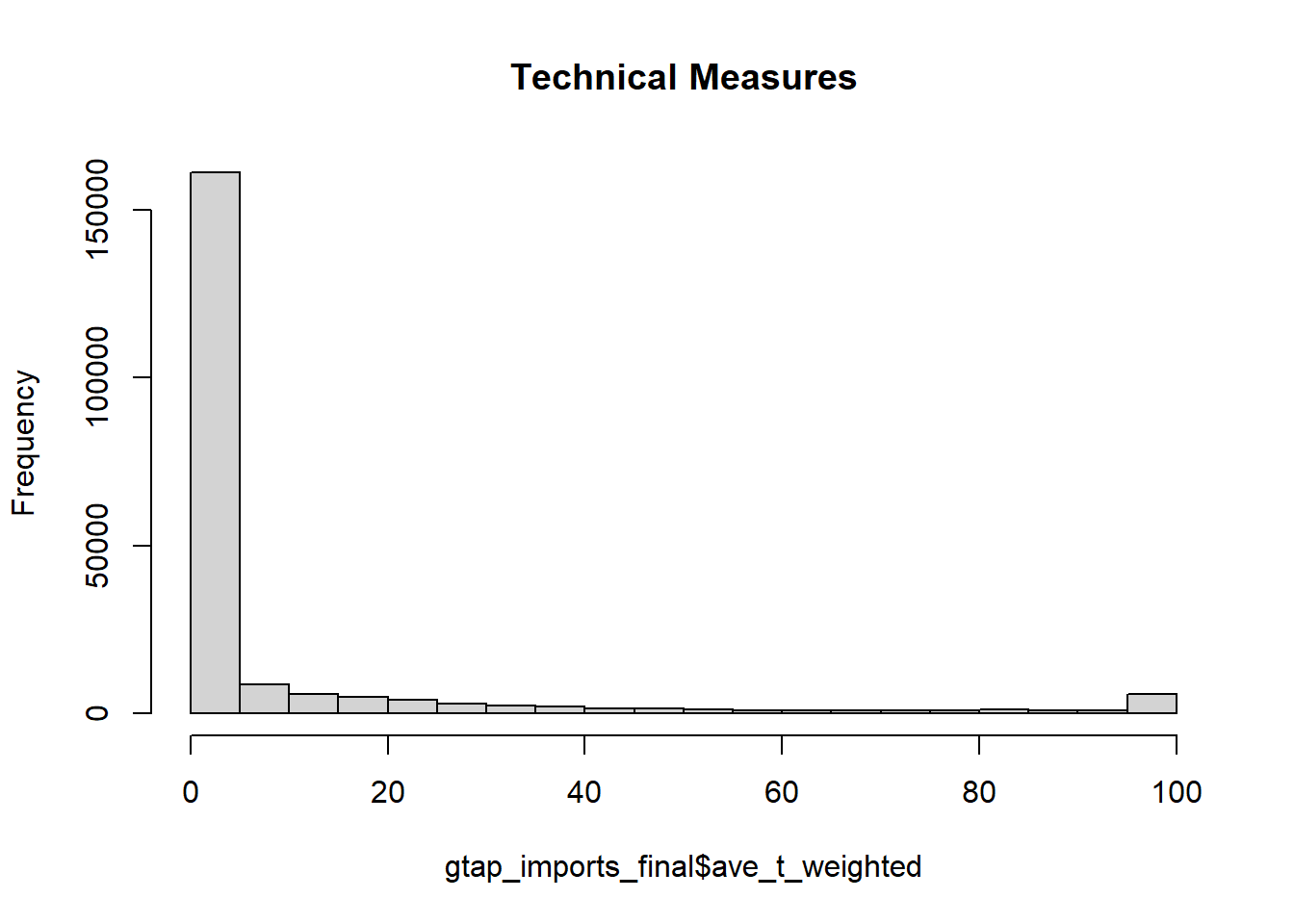
hist(gtap_imports_final$ave_nt_weighted, main = "Non-technical Measures")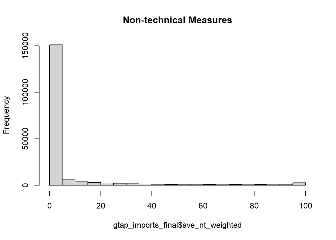
Congrats on making it this far! Any questions/suggestions/comments - please email kravchenkoa [at] un [dot] org