ESCAP Online Training on Using R for Trade Analysis
Introduction
This training material is designed to provide an introduction to trade analysis in R. There are 8 sections in total. The first four sections will provide you with some good basics for R, whereas sections 5, 6, 7 and 8 will focus on trade analysis. If you know how to program with R and are interested in trade analysis, we suggest you start from Section 5.
International trade is a key ingredient to economic growth, employment and poverty reduction. Being able to analyse trade data sets can help countries to understand better their trade with other countries and devise better policies. With the development of technologies now, there is more available data and easier access to it.
In our guide we explain how to perform analysis in R for gravity models (Section 5), Non-tariff Measures (NTMs) indicators (Section 6 & 7) and regulatory distance (Section 8). For these sections, basic statistical knowledge is required in order to be able to follow.
Gravity models are the backbone of applied international trade analysis and have been used in countless research papers. They are of particular interest for policy researchers because they provide insight into the relationship between trade flows and economic size and inversely with trade costs. This allows them to capture patterns in international trade and production. Policy researchers can use them to estimate the trade impacts of various trade-related policies, from traditional tariffs to new “behind-the-border” measures. If interested more in gravity models, we strongly suggest to review ESCAP’s original guide in STATA or the recent version in R.
NTMs have increased in number over the decade and currently have a bigger influence on trade than tariffs. Therefore, understanding their behavior and being able to assess how much of an influence they have on a country’s trade is crucial for policymakers. They can relate to the entire list of imports or be computed per product type. An example of an NTM is a temporary geographic prohibition of poultry imports or cattle from disease-affected countries. In this guide we will show how to compute three indicators using R: coverage ratio, frequency index and prevalence score. The coverage ratio (CR) measures the percentage of trade value subject to NTMs, the frequency index (FI) indicates the number of products in percentage to which NTMs apply, and the prevalence score (PS) is the mean number of NTMs per product(s). We discuss this in further detail in Section 6 and 7.
Regulatory distance (Section 8) is an indicator which measures the similarity between NTM policies across member States and sectors. This helps policymakers to assess the status quo of NTM-related regional integration and to benchmark progress. We display this information using multidimensional scaling, which shows how far or close countries are according to the regulatory distance. This helps visualize the distance between regional trade agreements.
What is R?
Let’s first begin with a short introduction on what is R?
R is an object orientated programming language and free software environment. You can perform data analytics, statistical and econometric models and visualization. Object-oriented programming is a type of computer programming in which:
- the programmer defines the type of an element or data set
- the programmer defines the type of functions to be applied on the element or data set
We will explain the different types of elements in R in Section 1. Every time we introduce a new function, we will highlight in blue the explanation.
To download R, we must go on the CRAN website and click on the version which applies to you - Linux, Mac or Windows.
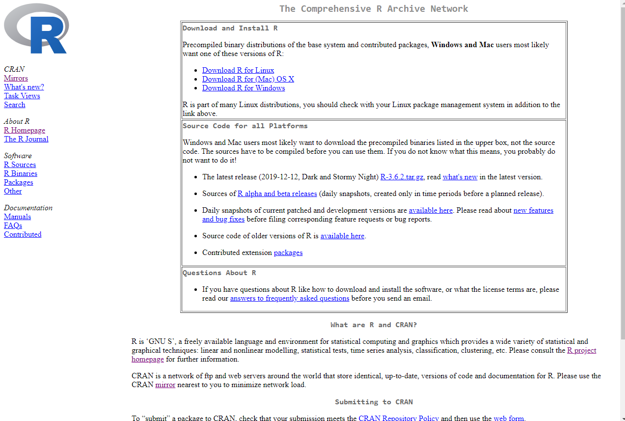
We choose Windows:
Once this is downloaded, click “Next” through everything and “Finish” at the end, and you’re done!
We can open R and run the code print("Hello!") by writing it in the console and pressing “Enter” like this:
You can see the output below the code.
We can select a new script, by clicking on “File” and choosing “New script” from the menu. We can print the phrase “Hello!” by typing print("Hello!") and right clicking “Run line or selection” or using the shortcut key “Control + R” or “Command + Enter” for Mac. The output will shows up in the console in red.
A better program to use R in, is R Studio. We can download it from the R Studio website. For the moment you can just choose the first option which is for free. We will use this version for the entire guide. Once again select for the operating system you have. We choose Windows.
Below is a simple demonstration of how to open a new script in R and run a sample code. As you can see the output shows up in the console (bottom left corner).
You can also run code by highlighting it with your mouse and pressing “Control + Enter” or “Command + Enter” for Mac.
Below is a small demonstration on creating variables, how to view plots, packages, help files and animations.
A package in R is a collection of functions which the user can call and run/use. R has the base package which is always automatically loaded, however packages developed by external users have to be downloaded and installed. Furthermore, in the beginning of each new R session, they have to be called from the library. Section 4.2 will demonstrate how to download the ggplot2 package, which is a very powerful package for making various types of plots and animations.
To load data, we can click on the “Import data set” in the upper right corner and select the type of file we want to upload. This will prompt a window to pop up where we select the folder in which the data is stored:
The usual way however is to set a working directory and take files from there. We will learn more about this in Section 2.
Now, let’s go into some code. No video is needed, you can straight away copy the code!
You will find quizzes in each section, which are not rated, but are simply designed to help you train and learn. Take your time with each section and make sure to complete all quiz questions. We strongly encourage for you to complete these quizzes as the questions resemble the survey questions to complete at the end for your certificate.
All the R code in the text is meant for you to run also on your own, provided that you have changed all the necessary paths. We recommend that you do each subsection at once in order to not lose track. If however you decide to do a section or subsection over two different session, we recommend you save your script and working environment. Each section introduces new comments and uses new data sets. The entire guide can take you from 2 weeks to a month if you devote a few hours every day, depending on your level (e.g. do you have programming experience or not).
When you start codes from the guide, save them in a script! This way it is easy to pick up where you left off! You can use this file which contains all the R codes from this guide.
We have started an R Cheat Sheet for you with the main commands, do include more commands as this will be especially helpful in the beginning to not forget what each command does! We will highlight in blue the explanations for any new command introduced.